README

About

Consider an image where some pixels/voxels show cortex and the rest indicate air. This program estimates the distance of each cortical voxel from air. Typical methods to do this use iterative erosion methods that are computationally intensive. This project uses the algorithm described by Felzenszwalb and Huttenlocher to solve this problem as a separable filtering problem. An excellent introduction to this problem and application is provided by Philip Rideout. Further, his Snowy project provides an elegant python implementation.

While Snowy is ideal for most situations, this project is specifically designed for high performance with medical images, reading various popular formats and saving distance fields in the popular NIfTI format, which you can view with many tools including MRIcroGL.

Installation

You can get Depth3D using two methods:

• (Recommended) Download latest compiled release from Github release web page.
• (Recommended) You can also download from the command line for Linux, MacOS and Windows:
  • curl -fLO https://github.com/neurolabusc/DistanceFields/releases/latest/download/Depth3D_lnx.zip
  • curl -fLO https://github.com/neurolabusc/DistanceFields/releases/latest/download/Depth3D_mac.zip
  • curl -fLO https://github.com/neurolabusc/DistanceFields/releases/latest/download/Depth3D_win.zip
• (Developers) Download the source code from GitHub.

Usage

Chris Rorden's Depth3D 64-bit (64-bit ints) MacOSv1.0.20191206
usage: Depth3D [options] <in_file(s)>
Reads volume and computes distance fields
OPTIONS
 -3 : save 4D data as 3D files (y/n, default n)
 -b : blur, specify full-width half maximum (positive=mm, negative=voxels, default 0)
 -c : connectivity neighbors (6=faces, 18=edges, 26=corners, default 26)
 -d : output datatype (u8/u16/f32 default f32)
 -h : show help
 -i : inverted mask image (ignore voxels with value of non-zero in mask)
 -k : mask image (ignore voxels with value of zero in mask)
 -o : output name (omit to save as input name with "depth_" prefix)
 -r : report table (y/n/s: yes, no, screen, default n)
 -t : threshold, less extreme values treated as outside (default 0.5)
       set to 0 for separate field for each region of an atlas
 -m : minimum cluster extent in voxels (default 1)
 -p : parallel threads (0=optimal, 1=one, 5=five, default 0)
 -s : save images (d,i,b,n: depth, intensity, both, none, default t) 
 -u : upsample for continuous images (1=x1, 5=x5 default 1)
       negative values for maximum of upsampled voxels.
 -z : gz compress images (y/n, default n)
 Examples :
  Depth3D -t 0 ./test/AICHA.nii.gz
  Depth3D -t 0 ./test/inia19-NeuroMaps.nii.gz
  Depth3D -t 0.5 ./test/4Dgraywhite.nii.gz
  Depth3D -t 0.5 ./test/isotropic.nii.gz
  Depth3D -t 0.25 -u 3 ./test/avg152T1_gray.nii.gz
  Depth3D -t 3 -m 5 -r s -s n ./test/motor.nii.gz
  Depth3D -k ./test/isotropic_mask.nii.gz ./test/isotropic.nii.gz
  Depth3D -o "~/out dir/OutputImg" -t 0.5 "./test/name with spaces"

Examples

Object Center

In this example, we compute the peak depth location for a C-shaped region. The image below shows that a nicely representative location has been identified. In contrast, the center of mass is outside the object.

Depth3D -t 0.5 -r y ./test/region4.nii.gz

Generates this table:

#VoxelVolume 1mm^3 (1x1x1)
#VolVox   MaxD x MaxD y  MaxD z MaxDpth   Label   CoG x   CoG y   CoG z     Max   Max x   Max y   Max z
  29345   31.00  -57.00  -15.00    7.35       1   20.85  -12.59   -3.34    1.00   33.00  -76.00  -12.00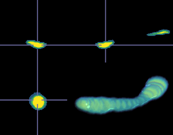

Sphere

It seems unintuitive that 3D thickness can be estimated by a separable filter that examines each line of each dimension sequentially. The image below shows axial, coronal and sagittal slices illustrating the thickness measures for a simple sphere. Note how well the thickness is modelled at off-axis angles.

Depth3D -t 0.5 ./test/isotropic.nii.gz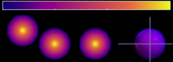

Atlas Centers

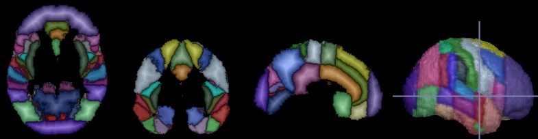
The image below shows the AICHA atlas in color, with the brightness modulated by the thickness of each of the 384 regions.

Depth3D -t 0  -r y ./test/AICHA.nii.gz

Generates the following report of centers:

#VolVox   MaxD x MaxD y  MaxD z MaxDpth   Label   CoG x   CoG y   CoG z
    139  -18.00   64.00   14.00    4.47       1  -15.99   64.94   13.08 
     25   12.00   68.00   10.00    2.83       2   12.88   67.68   10.64 
   1072  -14.00   50.00   38.00    4.90       3  -11.92   46.50   40.48 
   1113    8.00   48.00   44.00    5.66       4   12.04   45.58   40.70 
....

Masking

We can apply a mask to exclude voxels. The top panel in the image below shows an isotropic sphere (white) with a red bar-bell shaped mask (shown in red). Use -k to mask regions with zero value in the mask from our object. Use -i to apply an inverted mask. The mask is expected to be a 3D volume with identical shape and orientation with the primary image.

Depth3D -i ./test/isotropic_mask.nii.gz ./test/isotropic.nii.gz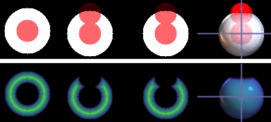

Up Sampling

This method assumes an image is binary: a voxel is either inside or outside the region. In reality, some voxels at the boundary of a region will be a mixture of the region and non-region. This is the partial volume problem: tissue is not constrained to respect the borders of our voxels. A nice example of this is tissue probability maps, where a voxel that is 75% gray matter and 25% other tissue (white matter, CSF) might have an intensity of 0.25. If we analyze this data at its original resolution, the results may be a bit blocky. One solution is to up-sample the data to a higher resolution, apply our threshold, compute thickness and downsample the resulting data. In theory, this method can capture some of boundary of the object a bit better. Thick3D provides the -u option that allows you to select a up-sampling factor. The image will be up-sampled and subsequently downsampled using a antialiasing Mitchell filter. Both the upsampling and the inherent smoothing of this filter can make the resulting values a bit less discrete. The images below were created with these two commands that compute thickness without super sampling (left) and with x4 supersampling (right).

Depth3D -t 0.25 ./test/avg152T1_gray.nii.gz
Depth3D -t 0.25 -u 4 ./test/avg152T1_gray.nii.gz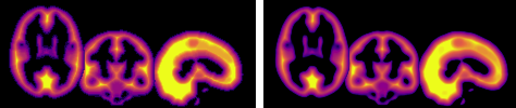

Culling Small Clusters

In the previous example, we applied an intensity threshold (e.g. -t 0.25), removing voxels darker that 0.25. We could also apply a second requirement, only keeping voxels that are both bright as well as being connected to a large group of bright voxels. Thick3D allows you to describe the minimum cluster volume (in mm3), which will remove smaller clusters. This can help eliminate noise spikes from our data, and is at the heart of Random Field Theory thresholding.

To identify large clusters, we need a definition of when two voxels are considered neighbors. Consider the image below where 4 voxels survive our intensity threshold (A,B,C,D). The crucial question is how many neighbors does voxel A have. If we only consider voxels that share a face, A has 6 neighbors one of which survives (B). These neighbors have a distance of one voxel between voxel centers. If we extend our definition to include the 12 neighbors that share an edge, we will count voxel C as part of the cluster as well. Neighbors that share an edge have a distance of 1.4 between voxel centers. Finally, if we include the eight voxels that share corners, we will include voxel D as part of the cluster. Corner voxels are separated by a distance of 1.7. Thick3D allows you to choose the neighbor method for faces (6 neighbors), faces and edges (18 neighbors) or faces, edges and corners (26 neighbors). These options are identical to the AFNI's 3dclust NNx, SPM's spm_bwlabel n and FSL's Cluster connectivity. Note that by default Thick3D and FSL use 26 neighbor connectivity while the SPM default is 18 (and AFNI requires you to always explicitly specify connectivity method).

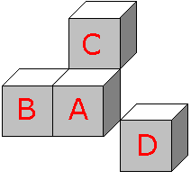
For example, lets look at voxels with an intensity greater than 3 that are part of clusters that have an extent of at least 5 voxels:

Depth3D -t 3 -m 5  -r s ./test/motor.nii.gz 
Removing clusters smaller than 5 voxels (40mm^3)
#VoxelVolume 8mm^3 (2x2x2)
#VolVox   MaxD x MaxD y  MaxD z MaxDpth   Label   CoG x   CoG y   CoG z     Max   Max x   Max y   Max z
    751  -40.00  -18.00   54.00    6.32       1  -33.46  -20.17   59.85    6.86  -40.00  -18.00   52.00 
     87   12.00  -30.00  -48.00    3.46       2   11.13  -30.71  -48.69    3.67   12.00  -28.00  -46.00 
     47  -26.00   50.00   20.00    3.46       3  -26.13   49.23   21.06    3.88  -24.00   48.00   22.00 
      9  -36.00   54.00   20.00    2.00       4  -36.00   53.56   20.22    3.23  -36.00   54.00   20.00 
      5   -4.00 -102.00    2.00    2.00       5   -4.00 -102.40    2.80    3.22   -4.00 -104.00    2.00

Assuming you have FSL installed you could run the analogous Cluster connectivity command.

cluster --in=./test/motor.nii.gz --thresh=3  --mm  --minextent=5
Cluster Index	Voxels	MAX	MAX X (mm)	MAX Y (mm)	MAX Z (mm)	COG X (mm)	COG Y (mm)	COG Z (mm)
5	751	6.86	-40	-18	52	-33.9	-20.1	59.7
4	87	3.67	12	-28	-46	11.1	-30.6	-48.7
3	47	3.88	-24	48	22	-26.1	49.2	21.1
2	9	3.23	-36	54	20	-36	53.6	20.2
1	5	3.22	-4	-104	2	-4	-102	2.8

By default, Thick3D generates thickness images as its output. However, the -s option allows you to specify the images saved. In this example, we might simply want to save the original input image after it has been thresholded small clusters have been culled. In this case we can use the -s i option to save the input image, or -s b to save both the thresholded input image and the cluster map. The image below shows the original image (top), the thresholded input (middle) and the thickness image (bottom) after the command

Depth3D -t 3 -m 5 -r s -s b ./test/motor.nii.gz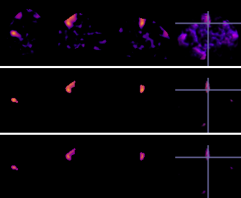

Limitations

• This software is provided as is. It uses the BSD license.
• Similar to erosion methods, this algorithm assumes that the spatial resolution is identical in each dimension. Anisotropic data must either be resliced to an isotropic grid or a different method must be used. This software uses the former approach, automatically up-sampling anisotropic images to be isotropic prior to thickness estimation, and subsequently downsampling the results to the original resolution.
• Similar to erosion methods, this traditional implementations of this algorithm assumes images are binary, which is not the case for probability maps. The Up Sampling example described previously attenuates but does not eliminate this limitation. William Silversmith provides an alternative approach for dealing with anisotropy.

Compiling

Most people will want to download a pre-compiled executable. Alternatively, Snowy provides a scriptable Python implementation. However, you can compile your own copy from source code:

• Download and install FreePascal for your operating system. For Debian-based unix this may be as easy as sudo apt-get install fp-compiler. For other operating systems, you may simply want to install FreePascal from the latest Lazarus distribution.
• From the terminal, go inside the directory with the source files and run the following commands to build and validate your compilation:

fpc Depth3D
./Depth3D -t 0 ./test/AICHA.nii.gz

Performance

This is a very fast algorithm. However, atlas images are necessarily complex, as depth is computed for each region independently. This tool uses several tricks that accelerate these cases. First, we can use a simple forward and back sweep for the first transformation. Second, depth is only computed for a box constrained by the size of the region being computed, rather than for the entire volume. This is useful for atlases with many regions, where each region typically is only a small portion of the overall 3D volume. In general, this trick makes the algorithm about 5 times faster. Finally, this algorithm can leverage parallel processing. The included sample AICHA atlas has 384 regions (91x109x91 voxels). It requires 1.7 seconds to process in single threaded mode and 0.43 seconds for threaded conversion on a 4-core (8-thread) laptop. Alternatively, consider a 512x512x512 voxel image converted with "Depth3D -u -3 maskedset.nii" - this requires 58 seconds on a 12-core (24-thread) Ryzen 3900X (14s upsample to 1536x1536x1536, 40s distance transform, 2s to downsample peaks to original resolution). The same machine running a single thread ("Depth3D -u -3 -p 1 maskedset.nii") requires 417 seconds (39s upsample, 361s transform, 14s downsample).

Supported Image Formats

Thick3D supports the same formats as i2nii:

• AFNI Brik(.head).
• Analyze(.hdr).
• Bio-Rad PIC(.pic).
• Blender Voxel data(.bvox).
• BrainVoyager VMR(.vmr, .v16).
• DeltaVision(.dv).
• ECAT(.v).
• FreeSurfer MGH/MGZ Volume(.mgh/.mgz).
• Guys Image Processing Lab(.gipl).
• ICS Image Cytometry Standard(.ics).
• Interfile(.varies, limited support).
• ITK MHA/MHD(.mha/.mhd).
• MRTrix Volume(.mif/.mih; not all variants supported).
• NIfTI(.hdr/.nii/.nii.gz/.voi). Useful for NIfTI-to-NIfTI modifications (e.g. -3, -d, -r, -z).
• NRRD(.nhdr/.nrrd).
• POV-Ray Density_File(.df3).
• Spectroscopic Imaging, Visualization and Computing (SIVIC)(.idf).
• Stimulate Sdt(.spr/.sdt)
• Vaa3D(.v3draw).
• VTK Legacy Voxel Format(.vtk).

If your image format is not supported, you may want to see if it is supported by the Bio-Formats module of ImageJ/Fiji. If so, you can open the image with the module and save it as NIfTI or NRRD.

Links

• Philip Rideout's distance fields page was the inspiration for this project. His snowy project provides distance fields (and more) for 2D images with a nice Python wrapper.
• William Silversmith's euclidean-distance-transform-3d provides optimized C code, Python wrappers, and comprehensive discussion of the origins and optimizations.