

neural-api

CAI NEURAL API - Pascal based deep learning neural network API optimized for AVX, AVX2 and AVX512 instruction sets plus OpenCL capable devices including AMD, Intel and NVIDIA.
- Active · last change 11-1-2026
- ★ 465 on GitHub
README
CAI NEURAL API
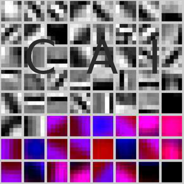
Everyone says Pascal died in the 90s. Meanwhile, this Pascal library runs GPT-style transformers, Mixture-of-Experts, RWKV, xLSTM, spiking neurons, and normalizing flows, natively, with no Python nor CUDA lock-in. Your PyTorch project: 4GB of dependencies, a conda environment that breaks monthly. This: compile to a single native binary with AVX. This is deep learning the way systems programmers wish it worked.
And it actually runs the real thing. Point the ChatTerminal example at a HuggingFace instruct model — Qwen2.5 (0.5B up to 32B), Qwen3, Qwen3.8, Llama (TinyLlama, SmolLM2), Mistral 7B, Phi-3-mini or the OLMoE Mixture-of-Experts — and chat with a genuine LLM in your terminal, or expose it as an OpenAI-compatible server with ChatServer: OpenCL-accelerated, no Python, no CUDA — with more architectures landing all the time. Then hand a text prompt to MusicGenText and watch the same library turn "lo-fi hip-hop with a mellow piano" into actual audio — T5 encoder and MusicGen decoder. One native binary, from a 20-line CIFAR demo to a billion-parameter transformer.
CAI NEURAL API is a Pascal deep-learning library optimized for the AVX, AVX2 and AVX512 instruction sets and for OpenCL devices from AMD, Intel and NVIDIA. Tested on Windows and Linux.
Highlights
- 🗣️ Run real LLMs, natively — import a HuggingFace instruct checkpoint (Qwen2.5/Qwen3/Qwen3.8, Llama, Mistral, Phi-3, OLMoE) and chat from your terminal with
ChatTerminal, or serve the same checkpoint over an OpenAI-style HTTP endpoint withChatServer, so any OpenAI client or SDK can call it. ChatServer'sPOST /v1/systemone(TypeSafe/Jev typed decisions: a state and typed questions in, option probabilities out, through the AnyJev L0 readout, or through a Kev / Open-Jev LoRA checkpoint with--decision-adapter) supports Open-Jev-2B (user-tested on itsQwen/Qwen3.5-2Bbase with--int4 --gpu); AnyJev L0, Kev and the other Open-Jev sizes are planned (coded). No Python, no CUDA. - 🎨 Text-to-image — turn a text prompt into a 1024x1024 image with
QwenImage(Qwen-Image-2.1: Qwen3-VL text encoder, 7B MMDiT transformer, VAE decoder; int8/int4 weights, OpenCL GPU by default). - 🎵 Text-to-music — turn a text prompt into audio with
MusicGenText(T5 encoder + MusicGen decoder). - 🔊 More audio — separate a song into stems with
MusicSourceSeparation, talk to an audio-aware model withQwen2AudioChat, or turn English text into speech withKokoroTTS(Kokoro-82M; a pure Pascal G2P reads misaki's dictionaries; REPL or one-shot). - 🧠 Modern architectures, built in — GPT-style transformers, Mixture-of-Experts, RWKV, xLSTM, spiking neurons and normalizing flows, all as native Pascal layers.
- 🖼️ Image super-resolution — upscale images with a trained network via the
SuperResolutioncommand-line tool (ships with a ready-to-use model). - ⚡ Fast everywhere — AVX/AVX2/AVX512 CPU paths plus OpenCL offload for AMD, Intel and NVIDIA GPUs.
- 📦 Single-binary deploy — compile to one self-contained native executable. No runtime, no dependency tree.
- 📖 Readable at native speed — clean, easy-to-learn Pascal that compiles to fast native code. No trade-off between readable source and raw performance.
Prerequisites
You'll need Lazarus development environment. If you have an OpenCL capable device, you'll need its OpenCL drivers. Many examples use the CIFAR-10 dataset. You'll also find examples for the CIFAR-100, MNIST, Fashion MNIST and the Places365-Standard Small images 256x256 dataset.
Will It Work with Delphi?
This project is Lazarus / Free Pascal based. The master branch does not work with Delphi. For Delphi, use v2.0.0 instead.
Installation
Clone this project, add the neural folder to your Lazarus unit search path and you'll be ready to go!
Documentation
The documentation covers:
- Easy examples
- Simple image classification examples
- Youtube videos
- Advanced examples
- Data structures (Volumes)
- Neural network layers
- Dataset support
- Training (fitting) your neural network
- Parallel computing
- Full set of examples
- Normalization Cheat Sheet
- Layer Authoring Guide — checklist for adding a new layer plus mini-guides on reading numerical-gradient failures and picking a tolerance
- Other scientific publications from the same author
Intro Videos
 |
 |
 |
|---|---|---|
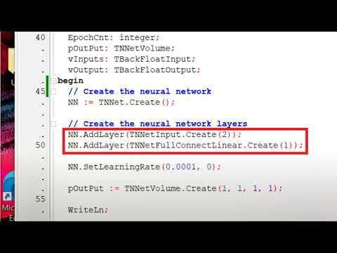
| Basics of Neural Networks in Pascal - Loading and Saving | Neural Networks for Absolute Beginners! Learning a Simple Function | Coding a Neural Network in Pascal that Learns to Calculate the Hypotenuse |
Easy Examples First Please!
You can click on the image above to watch the video.
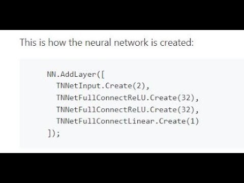
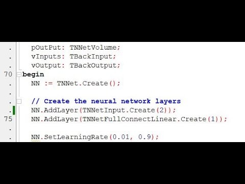
Assuming that you would like to train a neural network to learn a function that has 2 inputs and one output, you could start with something like this:
    NN.AddLayer([
      TNNetInput.Create(2),
      TNNetFullConnectReLU.Create(32),
      TNNetFullConnectReLU.Create(32),
      TNNetFullConnectLinear.Create(1)
    ]);
The example above has 2 inputs (TNNetInput), 2 dense layers (TNNetFullConnectReLU) with 32 neurons each and one output (TNNetFullConnectLinear).
You can learn more about how to build and train simple neural networks at the following source code examples:
- Only one neuron
- Training a neural network to learn the hypotenuse function
- Training a neural network to learn the hypotenuse function with FitLoading
- Training a neural network to learn boolean functions AND, OR and XOR with neuralfit unit
- Training a neural network to learn boolean functions AND, OR and XOR without neuralfit unit
- Reptile first-order meta-learning: learning an initialization that adapts to a new sine-regression task in a few SGD steps
- Lottery Ticket Hypothesis: magnitude-prune a small dense net, then retrain the sparse mask from the original init vs from fresh random weights — the original-init "winning ticket" matches the dense net and beats random reinit at moderate-to-high sparsity (pure CPU)
Loading and Saving Neural Networks
Loading is very easy:
    NN := TNNet.Create;
    NN.LoadFromFile('MyTrainedNeuralNetwork.nn');
Saving is as easy:
NN.SaveToFile('MyTrainedNeuralNetwork.nn');Simple Image Classification Examples
CIFAR-10 Image Classification Example
The CIFAR-10 dataset is a well-known collection of images commonly used to train machine learning and computer vision algorithms. It was created by the Canadian Institute for Advanced Research (CIFAR). It contains 60K 32x32 color images. The images are classified into 10 different classes, with 6,000 images per class. The classes represent airplanes, cars, birds, cats, deer, dogs, frogs, horses, ships, and trucks. Despite its relatively low resolution and small size, CIFAR-10 can be challenging for models to achieve high accuracy, making it a good dataset for testing advancements in machine learning techniques.
Follows a source code example for the CIFAR-10 image classification:
NN := TNNet.Create();
NN.AddLayer([
  TNNetInput.Create(32, 32, 3), //32x32x3 Input Image
  TNNetConvolutionReLU.Create({Features=}16, {FeatureSize=}5, {Padding=}0, {Stride=}1, {SuppressBias=}0),
  TNNetMaxPool.Create({Size=}2),
  TNNetConvolutionReLU.Create({Features=}32, {FeatureSize=}5, {Padding=}0, {Stride=}1, {SuppressBias=}0),
  TNNetMaxPool.Create({Size=}2),
  TNNetConvolutionReLU.Create({Features=}32, {FeatureSize=}5, {Padding=}0, {Stride=}1, {SuppressBias=}0),
  TNNetFullConnectReLU.Create({Neurons=}32),
  TNNetFullConnectLinear.Create(NumClasses),
  TNNetSoftMax.Create()
]);

CreateCifar10Volumes(ImgTrainingVolumes, ImgValidationVolumes, ImgTestVolumes);

WriteLn('Neural Network will minimize error with:');
WriteLn(' Layers: ', NN.CountLayers());
WriteLn(' Neurons:', NN.CountNeurons());
WriteLn(' Weights:', NN.CountWeights());

NeuralFit := TNeuralImageFit.Create;
NeuralFit.InitialLearningRate := fLearningRate;
NeuralFit.Inertia := fInertia;
NeuralFit.Fit(NN, ImgTrainingVolumes, ImgValidationVolumes, ImgTestVolumes, NumClasses, {batchsize}128, {epochs}100);
These examples train a neural network to classify images in classes such as: image has a cat, image has a dog, image has an airplane...
- Simple CIFAR-10 Image Classifier
- Simple CIFAR-10 Image Classifier with OpenCL
- Many neural network architectures for CIFAR-10 image classification
- MNIST, Fashion MNIST and CIFAR-100
You can save and load trained models (neural networks) with TNNet.SaveToFile and TNNet.LoadFromFile. The file format is portable meaning that you can train on CPU and run on GPU or train in AMD and run on ARM as examples. The following code shows a simple example for image classification loading a pre-trained model:
  procedure ClassifyOneImageSimple;
  var
    NN: TNNet;
    ImageFileName: string;
    NeuralFit: TNeuralImageFit;
  begin
    WriteLn('Loading Neural Network...');
    NN := TNNet.Create;
    NN.LoadFromFile('SimplePlantLeafDisease-20230720.nn');
    NeuralFit := TNeuralImageFit.Create;
    ImageFileName := 'plant/Apple___Black_rot/image (1).JPG';
    WriteLn('Processing image: ', ImageFileName);
    WriteLn(
      'The class of the image is: ',
      NeuralFit.ClassifyImageFromFile(NN, ImageFileName)
    );
    NeuralFit.Free;
    NN.Free;
  end;
Youtube Videos
|
|
|
|---|---|---|
| Basics of Neural Networks in Pascal - Loading and Saving | Neural Networks for Absolute Beginners! Learning a Simple Function | Coding a Neural Network in Pascal that Learns to Calculate the Hypotenuse |
 |
 |
https://youtu.be/o-8NuoSsdck |
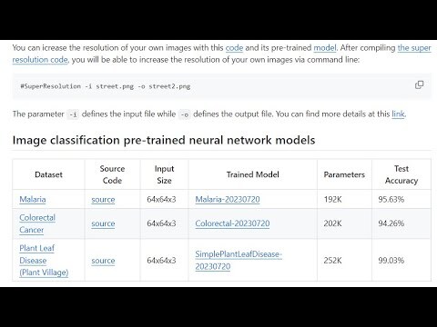
| Pre-trained Neural Networks & Transfer Learning with Pascal's CAI Neural API | Coding a Neural Network in Pascal that Learns the OR Boolean Operation | A Dive into Identity Shortcut Connection - The ResNet building block |
| https://youtu.be/SEvWB7k8uy0 | https://youtu.be/3QwIaAsDmJw | https://youtu.be/VH6v3D5cxxs |
| Increasing Image Resolution with Neural Networks | Ultra Fast Single Precision Floating Point Computing | AVX and AVX2 Code Optimization |
Some videos make referrence to uvolume unit. The current neuralvolume unit used to be called uvolume. This is why it's mentioned.
Advanced Examples
Although these examples require deeper understanding about neural networks, they are very interesting:
- Identity Shortcut Connection - ResNet building block
- ResNet-20 - includes a web server example
- DenseNetBC L40
- Separable Convolutions - MobileNet building block
- Gradient Ascent - Visualizing patterns from inner neurons in image classification
- Artificial Art - Let a neural network produce art via a generative adversarial network
- Super Resolution - A neural network learns how to increase image resolution
- CIFAR-10 Resized - A program that resizes CIFAR-10 and CIFAR-100 images to 64x64 and 128x128 pixels.
- Autoencoder - Shows an autoencoder built with hyperbolic tangents and trained with Tiny ImageNet 200.
There is also a full set of examples that you can look at.
Volumes
Volumes behave like dynamically created arrays. They are the main array like structure used by this API. TNNetVolume class allows you to create volumes that can be accessed as 1D, 2D or 3D arrays and be operated with Advanced Vector Extensions (AVX) - Single Instruction Multiple Data (SIMD) instruction set. The usual way to create a volume is:
constructor Create(pSizeX, pSizeY, pDepth: integer; c: T = 0);You can access the data as 1D or 3D with:
property Raw[x: integer]: T read GetRaw write SetRaw;
property Data[x, y, d: integer]: T read Get write Store; default;
Your code will look like this:
// Usage Examples
vInput := TNNetVolume.Create(32, 32, 3);
vInput[1, 1, 1] := 1;
vInput[2, 2, 2] := vInput[1, 1, 1] + 1;
vInput.Raw[10] := 5;

vInput.RandomizeGaussian();
WriteLn('Avg: ', vInput.GetAvg());
WriteLn('Variance: ', vInput.GetVariance());
WriteLn('Std Dev: ', vInput.GetStdDeviation());

WriteLn('Multiplying by 10');
vInput.Mul(10);
WriteLn('Avg: ', vInput.GetAvg());
WriteLn('Variance: ', vInput.GetVariance());
WriteLn('Std Dev: ', vInput.GetStdDeviation());
As examples, you can add, subtract, multiply and calculate dot products with:
procedure Add(Original: TNNetVolume); overload;
procedure Sub(Original: TNNetVolume); overload;
procedure Mul(Value: Single); overload;
function DotProduct(Original: TNNetVolume): TNeuralFloat; overload;
In the case that you need the raw position or raw pointer to an element of the volume, you can get with:
function GetRawPos(x, y, d: integer): integer; overload;
function GetRawPos(x, y: integer): integer; overload;
function GetRawPtr(x, y, d: integer): pointer; overload;
function GetRawPtr(x, y: integer): pointer; overload;
function GetRawPtr(x: integer): pointer; overload;
You can easily operate volumes with OpenCL via TEasyOpenCLV:
  TEasyOpenCLV = class (TEasyOpenCL)
    public
      function CreateBuffer(flags: cl_mem_flags; V: TNNetVolume): cl_mem; overload;
      function CreateInputBuffer(V: TNNetVolume): cl_mem; overload;
      function CreateHostInputBuffer(V: TNNetVolume): cl_mem; overload;
      function CreateOutputBuffer(V: TNNetVolume): cl_mem; overload;
      function CreateBuffer(V: TNNetVolume): cl_mem;  overload;

      function WriteBuffer(buffer: cl_mem; V: TNNetVolume; blocking: cl_bool = CL_FALSE): integer;
      function ReadBuffer(buffer: cl_mem; V: TNNetVolume; blocking: cl_bool = CL_TRUE): integer;

      function CreateAndWriteBuffer(V: TNNetVolume; var buffer: cl_mem): integer; overload;
      function CreateAndWriteBuffer(V: TNNetVolume): cl_mem; overload;
      function CreateWriteSetArgument(V: TNNetVolume; kernel:cl_kernel; arg_index: cl_uint): cl_mem;
      function CreateOutputSetArgument(V: TNNetVolume; kernel:cl_kernel; arg_index: cl_uint): cl_mem;
  end;
Volume Pairs, Volume Lists and Volume Pair Lists
Volumes can be organized in pairs:
  /// Implements a pair of volumes
  TNNetVolumePair = class(TObject)
    protected
      FA: TNNetVolume;
      FB: TNNetVolume;
    public
      constructor Create(); overload;
      constructor Create(pA, pB: TNNetVolume); overload;
      constructor CreateCopying(pA, pB: TNNetVolume); overload;

      destructor Destroy(); override;

      property A:TNNetVolume read FA;
      property B:TNNetVolume read FB;
      property I:TNNetVolume read FA;
      property O:TNNetVolume read FB;
  end;
Depending on the problem that you are trying to solve, modelling the training with pairs or pair lists might be helpful. Typically, a pair will be (input, desired output). This is how volume lists and volume pair lists have been implemented:
TNNetVolumeList = class (specialize TFPGObjectList<TNNetVolume>
TNNetVolumePairList = class (specialize TFPGObjectList<TNNetVolumePair>)
Neural Network Layers
The layered structure of artificial neural networks is inspired by the organization of the human brain and nervous system. In the human brain, information processing occurs in a hierarchical manner. Sensory inputs are first processed by lower-level neurons, which extract simple features. These features are then passed on to deeper neurons that combine them to recognize more complex patterns. This hierarchical processing is mirrored in artificial neural networks through the use of stacked layers.
Biological neurons are connected to each other through synapses, forming complex networks. Similarly, in artificial neural networks, neurons in one layer are connected to neurons in the next layer, mimicking this interconnected structure. Biological neurons fire (activate) based on a non-linear response to their inputs. This non-linearity is crucial for the brain's ability to learn complex patterns. In artificial neural networks, we use non-linear activation functions (such as ReLU) to introduce this non-linearity. Different regions of the brain specialize in processing different types of information. For instance, the visual cortex has layers specialized for detecting edges, shapes, and complex objects. This specialization is reflected in artificial neural networks, where different layers can learn to recognize different levels of abstraction.
In the context of artificial neural networks, we can see this biologically-inspired layered approach implemented. For example:
NN := TNNet.Create();
NN.AddLayer([
  TNNetInput.Create(32, 32, 3),
  TNNetConvolutionLinear.Create({neurons=}16, {featuresize}3, {padding}1, {stride}1),
  TNNetReLU6.Create()
]);
This code snippet demonstrates the creation of a neural network with an input layer and a convolutional layer followed by a ReLU6 activation. This structure is inspired by the visual cortex in the brain, where neurons respond to specific patterns in their receptive fields, similar to how convolutional layers operate. The CAI Neural API also supports the creation of more complex, biologically-inspired architectures. These architectures are designed with multiple layers of different types, mirroring the complex structure of the brain.
Artificial neural networks with multiple layers and specialized structures are inspired by the hierarchical and specialized nature of biological neural processing. It's important to note that while artificial neural networks are inspired by biological neural networks, they are highly simplified models. The human brain is far more complex, with various types of neurons, complex connectivity patterns, and mechanisms we don't yet fully understand. However, the layered structure in artificial neural networks has proven to be a powerful approach for solving complex problems in machine learning, inspired by the remarkable capabilities of biological neural networks.
Input Layer
The input layer serves as the gateway to the entire network. It's like the sensory organs of our brain, receiving information from the outside world. Without an input layer, the neural network would have no way to receive and interpret the initial data, making it impossible to perform any meaningful computations or learning tasks. The TNNetInput class implements the input layer.
Fully Connected (Dense) Layers
Fully connected layers, also known as dense layers, are a fundamental component of neural networks. In these layers, every neuron is connected to every neuron in the previous layer, allowing for comprehensive information processing across the entire network.
In the context of the CAI Neural API, fully connected layers are represented by various classes derived from TNNetFullConnect. These layers play a crucial role in transforming input data and learning complex patterns.
The computation process in a fully connected layer involves:
- Multiplying input values by the layer's weights.
- Adding bias terms (if not suppressed).
- Applying an activation function (if present).
Key types of fully connected layers include:
TNNetFullConnectLinear: a basic fully connected layer without an activation function. It performs a linear transformation of the input data.TNNetFullConnectReLU: incorporates the Rectified Linear Unit (ReLU) activation function. ReLU introduces non-linearity by outputting the input for positive values and zero for negative values, helping the network learn complex patterns.TNNetFullConnectSigmoid: applies the sigmoid activation function to the layer's output. Sigmoid squashes the output between 0 and 1, useful for binary classification tasks.TNNetComplexLinear: the 2-dimensional complex base rung of the same Cayley–Dickson family — each 2-channel group(Re,Im)is multiplied by a learned complexw = a + b·ivia the 2×2 complex-multiply block[[a,-b],[b,a]](Re' = a·Re − b·Im,Im' = a·Im + b·Re), using ~1/2 the weights of an equal-width real dense layer while still mixing the real and imaginary parts. The forward block equals the true complex product and is norm-multiplicative|w·X| = |w|·|X|. Input/outputDepthmust be multiples of 2. Seeexamples/ComplexLinear/.TNNetQuaternionLinear: a hypercomplex dense layer that shares each 4×4 Hamilton block from a single learned quaternion, coupling 4-channel groups (rotation/scaling in quaternion space) with ~1/4 the weights of an equal-width real dense layer. Input/outputDepthmust be multiples of 4.TNNetOctonionLinear: the 8-dimensional octonion (Cayley–Dickson) generalization of the above — each 8-channel group is multiplied by a learned octonion via the (non-associative) octonion product, assembled as an 8×8 signed block, using ~1/8 the weights of an equal-width real dense layer. The implementation hard-codes an auditable Cayley–Dickson sign table verified by a norm-multiplicativity test (|W·X| = |W|·|X|). Input/outputDepthmust be multiples of 8. Seeexamples/OctonionLinear/.
Fully connected layers are typically used in neural network architectures as:
- Hidden layers for processing and transforming features.
- Output layers for producing final predictions.
For example, in the provided context, we see a simple neural network structure:
NN := TNNet.Create();
NN.AddLayer([
  TNNetInput.Create(2),       // Input layer with 2 inputs
  TNNetFullConnect.Create(2), // Hidden fully connected layer with 2 neurons
  TNNetFullConnect.Create(1)  // Output fully connected layer with 1 neuron
]);| Layer Name | Input/Output Dimensions | Activation | Description |
|---|---|---|---|
TNNetFullConnectLinear |
1D, 2D, or 3D | None | Fully connected layer without an activation function (linear). |
TNNetFullConnect |
1D, 2D, or 3D | tanh | Fully connected layer with tanh as the default activation function. |
TNNetFullConnectReLU |
1D, 2D, or 3D | ReLU | Fully connected layer with ReLU activation. |
TNNetFullConnectSigmoid |
1D, 2D, or 3D | Sigmoid | Fully connected layer with Sigmoid activation. |
TNNet.AddGroupedFullConnect |
1D, 2D, or 3D | Optional | Adds a grouped fully connected layer, inspired by TNNet.AddGroupedConvolution. |
TNNetBitLinear |
1D, 2D, or 3D | None | BitNet b1.58 ternary-weight linear layer: forward uses per-neuron absmean-quantized weights Wq = scale*round(clip(W/scale,-1,+1)) with `scale = mean( |
TNNetCirculantLinear |
1D, 2D, or 3D (n=Depth) |
None | Structured-matrix dense layer whose n×n weight matrix is CIRCULANT — every row is a cyclic shift of one learned length-n kernel c, so it stores O(n) weights instead of O(n²) and the map is y = circular_convolution(c, x) (+ bias). Default forward/backward is the exact direct O(n²) circular sum; set UseFFT := true for an opt-in O(n log n) radix-2 FFT fast path (power-of-two n; default OFF, bit-for-bit equivalent to the direct path to <1e-5). Distinct from LoRA (low-rank), AddGroupedFullConnect (block-diagonal) and TNNetBitLinear (quantized dense). See examples/CirculantLinear/. |
TNNetHouseholderLinear |
1D, 2D, or 3D (n=Depth) |
None | EXACTLY-orthogonal dense layer whose n×n weight is parameterized as a product of K Householder reflections Q = H_1·H_2·…·H_K with H_i = I − 2·(v_i·v_iᵀ)/(v_iᵀ·v_i); the trainable parameters are the K reflection vectors v_i ∈ ℝ^n. Q is orthogonal for any v_i (no constrained optimization or re-projection), so the map is exactly norm/volume preserving (‖y‖ = ‖x‖ with bias off) and exactly invertible (Qᵀ = H_K·…·H_1). Forward applies the reflections one at a time (O(K·n) per sample, never materializing Q), y = Q·x (+ bias); backward caches each intermediate x_i = H_i·…·H_K·x for a closed-form per-v_i gradient and propagates dL/dx = Qᵀ·dL/dy. An exactly-orthogonal Jacobian is an isometry, so deep plain stacks neither explode nor vanish (the building block for orthogonal/unitary RNNs and reversible/normalizing-flow nets). Distinct from TNNetSpectralNorm (bounds only σ_1, leaves the other singular values free), TNNetCirculantLinear/Toeplitz (constrain the matrix form, not orthogonality) and Muon (orthogonalizes the update, not the weight). The v_iᵀ·v_i → 0 denominator is guarded (degenerate reflection ≈ identity). Composite helper TNNet.AddHouseholderLinear(N, NumReflections, UseBias) (default K = n for a full orthogonal group element; K < n gives a cheaper sub-group). See examples/HouseholderOrthogonal/. |
TNNetHyperbolicLinear |
1D, 2D, or 3D (Depth-vector point in the ball) |
None | Poincaré-ball HYPERBOLIC dense layer (Ganea, Bécigneul & Hofmann 2018, Hyperbolic Neural Networks; Nickel & Kiela 2017): treats the Depth-vector input x as a point inside the open Poincaré ball of radius 1/√c (fixed curvature c>0, default 1.0) and computes the Möbius matrix–vector product followed by a hyperbolic (Möbius) bias translation, y = exp_0(M·log_0(x)) ⊕_c b, where log_0(x)=(1/√c)·atanh(√c‖x‖)·x/‖x‖ and exp_0(v)=(1/√c)·tanh(√c‖v‖)·v/‖v‖ are the log/exp maps at the origin and a ⊕_c b is Möbius addition. Reuses the TNNetFullConnectLinear weight layout (one neuron per output dim holds matrix row M[j]; the Möbius bias b is held coordinate-wise in the per-neuron bias). Genuinely non-Euclidean — unlike every other dense layer here (all flat sum_j W·x plus optional Euclidean bias), the matmul and bias act in hyperbolic space, the natural geometry for embedding trees / hierarchies with low distortion; the output always stays inside the ball (‖y‖<1/√c). Backward is the EXACT analytic chain rule through both radial atanh/tanh maps and the Möbius-addition Jacobian (input, matrix-row and Möbius-bias gradients all numerically gradient-checked); the ‖x‖→1/√c boundary and ‖x‖→0 origin are guarded by an EPS/series fallback so the Jacobian stays finite. Curvature c round-trips via FFloatSt[0]; suppress-bias via FStruct[3]. Created with TNNetHyperbolicLinear.Create(Dout) (default c=1) or Create(Dout, c). Optional trainable curvature: Create(Dout, c, SuppressBias, LearnCurvature:=true) makes c a single learnable scalar via the constrained-scalar pattern — one extra 1-weight neuron holds a raw value mapped through c = 0.01 + 3.99*sigmoid(raw) (kept strictly positive/bounded), the exact dL/draw is accumulated via a forward-mode tangent of y through the log_0/exp_0/Möbius-add chain, and the flag round-trips via FStruct[4]. The default (fixed-c) path is byte-for-byte unchanged. |
TNNetHyperbolicDistance |
1D, 2D, or 3D (Depth-vector point in the ball) |
None | Poincaré-ball distance READOUT head (companion to TNNetHyperbolicLinear): maps the Depth-vector input x (a point inside the curvature-c Poincaré ball) to a K-vector of hyperbolic distances to K learnable prototype points p_k, d_k = dist_c(x, p_k) = (2/√c)·atanh(√c·‖(-x) ⊕_c p_k‖) (Möbius addition ⊕_c as in TNNetHyperbolicLinear). Reuses the TNNetFullConnectLinear weight layout (one neuron per prototype holds p_k, bias suppressed). A usable hyperbolic classification/regression head — small distances mean "close in hyperbolic space". Backward is the EXACT analytic chain rule through the radial atanh and the Möbius-addition Jacobian (input and per-prototype gradients both numerically gradient-checked); boundary/origin guarded by EPS/series fallback. Curvature c round-trips via FFloatSt[0], prototype count K via FStruct[0]. Created with TNNetHyperbolicDistance.Create(K) (default c=1) or Create(K, c). See examples/HyperbolicEmbedding/. |
TNNetMonarchLinear |
1D, 2D, or 3D (n=Depth) |
None | Sub-quadratic STRUCTURED dense layer whose n×n weight is a MONARCH matrix (Dao et al. 2022, Monarch: Expressive Structured Matrices for Efficient and Accurate Training): a product of two block-diagonal factors interleaved by a fixed reshape-transpose permutation, y = Pᵀ·(L·(P·(R·x))) (+ bias), where R and L are block-diagonal with b blocks of size m×m (n = b·m, default b = round(√n) for perfect-square n, else the largest divisor ≤ √n; b round-trips via FStruct[1]) and P is the fixed (b,m)→(m,b) index-gather permutation (no weights). Stores/runs in O(n^1.5) instead of O(n²) yet provably contains the DFT, the Hadamard transform and ordinary convolutions — a genuinely different structured operator from TNNetCirculantLinear (single cyclic kernel), LoRA (low-rank) and AddGroupedFullConnect (one block-diagonal, no permutation mix). Forward applies R, permute, L, un-permute as four cheap passes (never materializing the dense n×n); backward is the exact transpose chain (dL/dx, dL/dR, dL/dL all block-local matmuls), both factor gradients numerically gradient-checked. Suppress-bias via FStruct[3]. The map is square, so n is inferred from the previous layer's size; created with TNNetMonarchLinear.Create() (or Create(1) to suppress bias). |
TNNetKroneckerLinear |
1D, 2D, or 3D (n=Depth) |
None | Sub-quadratic STRUCTURED dense layer whose n×n weight is a single KRONECKER PRODUCT W = A ⊗ B of two small learned factors A (p×p) and B (q×q) with n = p·q. Stores only O(p²+q²) ≈ O(n) weights instead of O(n²), and the dense n×n Kronecker matrix is NEVER materialized: x is reshaped to a q×p matrix X (X[i,j] = x[i·p+j]) and the matvec is two small GEMMs Y = B·X·Aᵀ (O(n·(p+q)) = O(n^1.5)), flattened back as y[i·p+j] = Y[i,j] (+ bias). Under this row-major vec convention y = vec(B·X·Aᵀ) exactly equals (A⊗B)·x. Backward is the exact transpose chain dL/dX = Bᵀ·dY·A, dL/dA = dYᵀ·(B·X), dL/dB = dY·(X·Aᵀ)ᵀ (all small GEMMs; input, dA and dB all numerically gradient-checked). The factor split p defaults to round(√n) (largest divisor ≤ √n when n is not a perfect square) and round-trips via FStruct[1]; q = n div p. A genuinely different structured operator from TNNetCirculantLinear (single cyclic kernel), TNNetHouseholderLinear (exactly orthogonal), TNNetMonarchLinear (two block-diagonal factors + permutation) and LoRA (low-rank): Kronecker is a single tensor-product factorisation. Suppress-bias via FStruct[3]. The map is square, so n is inferred from the previous layer's size; created with TNNetKroneckerLinear.Create() (or Create(1) to suppress bias, or Create(0, p) to pin the factor split). See examples/KroneckerLinear/. |
TNNetTropicalLinear |
1D, 2D, or 3D (Din=Depth) |
None | A max-plus / min-plus morphological dense layer that computes in the TROPICAL (max-plus) semiring instead of the usual multiply-accumulate ring: y_i = max_j (x_j + W[i,j]) (a morphological DILATION), with a paired ERODE mode y_i = min_j (x_j + W[i,j]) selected by a constructor flag (round-trips via FStruct[6]). The weights are learnable additive thresholds and the combine op is max/min, so the layer learns piecewise-linear convex (dilation) / concave (erosion) functions and tropical polynomials — a genuinely different operator from TNNetFullConnect* and the structured-linear family (TNNetCirculantLinear/TNNetHouseholderLinear/TNNetBitLinear, all sum_j W·x) and from parameter-free max/min pooling. Forward is O(Din·Dout); backward is the same hard arg-max/arg-min subgradient as TNNetMaxPool — cache the winning j* per output and route dL/dx[j*] += dy_i, dL/dW[i,j*] += dy_i (non-differentiable at ties). Both the input and weight gradients are numerically gradient-checked (away from the tie kink). Created with TNNetTropicalLinear.Create(Dout) (dilation) or Create(Dout, 1) (erode). See examples/TropicalMorphology/. |
TNNetTropicalConv |
2D or 3D (SizeX x SizeY x Depth) | None | The SPATIAL sibling of TNNetTropicalLinear — a grayscale morphological dilation/erosion convolution with a learnable additive structuring element (SE) over a (SizeX,SizeY,Depth) patch: y[x,y,co] = max_{dx,dy,ci} (input[x+dx,y+dy,ci] + SE[dx,dy,ci,co]) (dilation), with a paired ERODE mode min_{dx,dy,ci} (input − SE) selected by a constructor flag (round-trips via FStruct[6]). Subclasses TNNetConvolutionLinear for the conv geometry (kernel/padding/stride) but replaces the multiply-accumulate with the max-plus/min-plus semiring and a single SE weight neuron — distinct from parameter-free TNNetMaxPool (learnable additive SE, not a fixed window) and from ordinary linear conv (sum W·x). Backward is the hard arg-max/arg-min one-hot subgradient (MaxPool convention): cache the winning (dx,dy,ci) tap per output cell and route dy to that single input cell and that single SE tap (non-differentiable at ties). Both input and SE gradients numerically gradient-checked (away from the tie kink). Created with TNNetTropicalConv.Create(Features, FeatureSize, Padding, Stride) (dilation) or Create(Features, FeatureSize, Padding, Stride, 1) (erode). |
TNNetCondConv |
2D or 3D (SizeX x SizeY x Depth) | None | Conditionally-parameterized ("dynamic") convolution (Yang et al. 2019, CondConv, NeurIPS): owns a bank of K expert kernels W_1..W_K (each a normal Features × FeatureSize × FeatureSize × InChannels kernel) plus a tiny per-sample routing head (global-average-pool → FullConnect → sigmoid) emitting K mixing coefficients alpha_k per input sample; the effective kernel is the per-sample blend W_eff = sum_k alpha_k·W_k applied as ONE ordinary convolution — so inference cost stays that of a single conv regardless of K while capacity grows with the bank. Backward routes dL/dW_k = alpha_k·dL/dW_eff, sends dL/dalpha_k = <dL/dW_eff, W_k> back through the sigmoid + FC + pool into the input, and propagates the standard conv input gradient through W_eff (input, expert-bank, and routing-head gradients all numerically gradient-checked). Distinct from TNNetHyperConv (GENERATES the whole kernel from a second tensor in one shot) and AddMixtureOfExperts (mixes K expert OUTPUTS post-hoc, K forward passes); CondConv mixes K kernels BEFORE the conv (one forward pass). K/Features/FeatureSize/Padding/Stride round-trip via FStruct. Created with TNNetCondConv.Create(K, Features, FeatureSize, Padding, Stride). See examples/CondConv/. |
TNNetSpectralNorm |
1D, 2D, or 3D | None | Spectral-normalized dense layer (Miyato et al. 2018): forward divides the weight matrix by its largest singular value sigma_1 (estimated by power iteration, Iters steps in FStruct[5], default 10) so the effective operator W/sigma_1 has spectral norm ~1; sigma_1 is treated as constant in backward (input error propagated through the scaled weights). |
TNNetHighway |
1D, 2D, or 3D (shape-preserving over Depth) |
Optional | Highway-network layer (Srivastava, Greff & Schmidhuber 2015): y = T(x)⊙H(x) + (1−T(x))⊙x with an input-dependent transform gate T(x) = sigmoid(W_T·x + b_T) and learned transform H(x) = activation(W_H·x + b_H). The input-dependent learned-gate ancestor of the ResNet skip connection — unlike TNNetReZero (scalar) and TNNetGatedResidual (per-channel constant), the gate is computed from the activation each forward pass and carries the identity (1−T)·x. Gate bias inits negative (b_T ≈ −1.5, the paper's carry trick) so a fresh deep stack starts near identity. Per-channel pointwise, so it composes inside the residual builders. See examples/HighwayDepth/. |
TNNetHyperLinear |
main: 1D/2D/3D → Dout |
None | HyperNetwork dense layer (Ha, Dai & Le 2016): owns NO trainable weights — its weight matrix is GENERATED by an upstream net and read from a SECOND input tensor (WeightsSource, a flat Din*Dout (+Dout) row-major matrix + optional bias) rather than from Neurons[]. Two-source wiring like TNNetCrossAttention. Forward y = W_gen·x (+b); backward propagates into BOTH the main input (W_gen^T·dy) and the generated-weights tensor (dy⊗x, dy) so the generator trains end-to-end. Composite helper TNNet.AddHyperLinear(Din, Dout, ContextLayer, UseBias=true) wires the generator FullConnect (off ContextLayer) and the weightless TNNetHyperLinear (off the main path) in one call. See examples/HyperNetwork/. |
TNNetHyperConv |
main: 3D image → VALID conv | None | Spatial cousin of TNNetHyperLinear — a weightless convolution whose kernel is GENERATED by an upstream net and read from a SECOND input tensor instead of Neurons[]. VALID conv, stride 1; kernel laid out W[o,ky,kx,i] flat (((o*K+ky)*K+kx)*InChannels + i) plus optional per-output-channel bias. Backward propagates into BOTH the main image and the generated-kernel tensor so the generator trains end-to-end. Composite helper TNNet.AddHyperConv(InChannels, OutChannels, FeatureSize, ContextLayer, UseBias=true) wires the generator FullConnect and the weightless TNNetHyperConv in one call. Note: the generator emits the whole OutC*K*K*InC kernel in one shot, which caps kernel/channel size (memory/param trade-off). |
TNNetModulatedConv2D |
main: 3D image → SAME conv | Conv kernel (+bias) | StyleGAN2 weight-modulated / demodulated convolution (Karras et al. 2020, Analyzing and Improving the Image Quality of StyleGAN) — the style-synthesis PRIMITIVE, a WEIGHT-SPACE op (not an activation). Unlike TNNetHyperConv (whose whole kernel is generated upstream) this OWNS a trainable base kernel in Neurons[] and per forward pass SCALES it by a per-input-channel style vector read from a SECOND input then RENORMALIZES: modulate w'[o,k,i]=s_i·w[o,k,i], demodulate w''[o,k,i]=w'[o,k,i]/sqrt(Σ_{k,i} w'^2 + ε) (toggle off for the toRGB 1×1 conv). SAME padding, stride 1; backward routes gradient to the owned kernel (through the demod normalization, dd/dw'=-d^3·w'), the feature input, AND the style branch (so the mapping/affine trains end-to-end). Two-source wiring like TNNetHyperConv (Create(NumFeatures, FeatureSize, SuppressBias, Demodulate, StyleSource)); FStruct + the injected style-source index round-trip through SaveToString. Used by BuildStyleGAN2Generator (neuralpretrained.pas). See examples/StyleGAN2Generate/. |
TNNetModernHopfield |
2D (SeqLen x 1 x d) |
Pattern bank | Modern continuous Hopfield associative-memory layer (Ramsauer et al. 2020, Hopfield Networks is All You Need): an ENERGY-BASED memory that ITERATES a softmax retrieval to a fixed point against a learnable stored-pattern bank X of shape (NumPatterns, d). Per query position, xi := X^T·softmax(beta·X·xi) is applied for K update steps — K=1 reduces to ordinary attention, K>1 sharpens toward the nearest stored memory (the whole point). Inverse-temperature beta controls the metastable-vs-sharp regime. Forward caches per-step softmax weights; backward differentiates through the unrolled K steps (the SDPA softmax-Jacobian path, summed over steps, scattered into both bank and input). Composite helper TNNet.AddModernHopfieldRetrieval(NumPatterns, KSteps, Beta) wires a (SeqLen,1,d) query against a fresh learnable bank. See examples/HopfieldAssociativeMemory/. |
TNNetProductKeyMemory |
Input: SeqLen x 1 x QueryDim (even QueryDim, divisible by Heads with QueryDim/Heads even). Output: SeqLen x 1 x (Heads*ValueDim). |
Half-keys + values (per head) | Large, sparsely-accessed product-key memory (Lample et al. 2019, Large Memory Layers with Product Keys): factorizes a NumKeys-row memory into the Cartesian product of two small half-key banks K1, K2 (each sqrt(NumKeys) rows of (QueryDim/Heads)/2). A query is split in half, each half scored against its own bank, the top-TopK per half taken, the TopK x TopK combinations re-scored, and the global top-TopK product keys selected in O(sqrt(NumKeys)) work; a softmax over those gates a sparse weighted sum over only the touched rows of the learned value table. Multi-head (Heads>1): the query is split into Heads contiguous sub-queries, each running an independent product-key lookup against its own K1/K2/V banks (3*Heads neurons; head h owns neurons 3h,3h+1,3h+2), and the Heads ValueDim-wide outputs are concatenated along Depth. Heads=1 is byte-for-byte the v1 single-head path. Forward caches the chosen indices + weights; backward scatters the value-gradient into only the touched value rows and pushes the exact softmax-Jacobian score-gradient back through both half-key dot products into the query and K1/K2. Distinct from TNNetModernHopfield (dense softmax over a small fully-retrieved bank), TNNetEmbedding (one-hot lookup), and MoE (expert MLPs). Composite helper TNNet.AddProductKeyMemory(NumKeys, ValueDim, TopK, Heads). See examples/ProductKeyMemory/. |
TNNetNTMMemory |
Input: T x 1 x InputDim. Output: T x 1 x SlotWidth (per-step read vectors). |
Key/beta/erase/add projections | The first writable differentiable external-memory layer in the library — a Neural Turing Machine (Graves et al. 2014, Neural Turing Machines, arXiv:1410.5401). Unlike the read-only associative memories (TNNetModernHopfield iterated recall, TNNetProductKeyMemory sparse lookup) it carries a persistent memory matrix M (NumSlots × SlotWidth) that the layer both reads and writes while sweeping the time axis. Per step the input is projected to a content key (cosine-addressed against every slot row, sharpened by a softplus key-strength beta, softmaxed over slots → weights w), a read r_t = w^T·M (the step's output), and a sigmoid erase e + add a that update M[i] := M[i]·(1 − w[i]·e) + w[i]·a (erase-then-add, same w). The four projection matrices (8 neurons Wk,bk,Wb,bb,We,be,Wa,ba) are the only trainables; backward is full BPTT through the recurrent M update — because M_t depends on both M_{t-1} and w_t, dL/dM and dL/dw both chain backward across steps (input, read-path and write-projection gradients all numerically gradient-checked). NumSlots/SlotWidth round-trip via FStruct[0..1], InitVal via FFloatSt[0]; M is re-initialised to a small constant each sweep and is not persisted across loads (re-init on load, like SetAdjacency). v1 is content addressing only, single read+write head; location-based shift/interpolation addressing and the DNC temporal-link matrix are documented follow-ups. Created with TNNetNTMMemory.Create(NumSlots, SlotWidth, InitVal=0.001). See examples/NeuralTuringMachine/. |
TNNetSoftDecisionTree |
Input: flat Din-vector. Output: 1 x 1 x OutputDepth. |
None (mixture of leaf vectors) | Differentiable soft (oblique) decision tree (Kontschieder et al. 2015, Deep Neural Decision Forests; Frosst & Hinton 2017, Distilling a Neural Network Into a Soft Decision Tree) — a structurally new hierarchical soft-routing paradigm for this library (not a matrix factorization, attention, recurrence or kernel method). A balanced binary tree of fixed depth D has 2^D−1 inner nodes and 2^D leaves. Each inner node i is a learnable linear gate p_i = sigmoid(beta·(w_i·x + b_i)); a sample reaches a leaf with probability equal to the product of the left (p_i) / right (1−p_i) gate decisions along its root-to-leaf path, and the output is the path-probability-weighted mixture `y = sum_l P(leaf=l |
TNNetGridSample |
main: 3D feature map SizeX x SizeY x Depth; second source: dense SizeX x SizeY x 2 normalized grid (x_n, y_n) in [-1,1] (same spatial size). Output: same shape as the features. |
None (pure differentiable resampling) | Faithful port of torch.nn.functional.grid_sample (4-D case) — a two-source layer that warps the feature map by an EXPLICIT per-output-pixel sampling grid. Unlike TNNetAffineGridSample (grid from one global 2×3 theta) or TNNetFlowWarp/TNNetBackwardWarp (PIXEL-unit (dx,dy) flow), the grid here gives normalized [-1,1] sample coordinates over the output grid, exactly the torch convention. Supports mode='bilinear' (gsiBilinear) / 'nearest' (gsiNearest), padding_mode='zeros' (gspZeros) / 'border' (gspBorder), and the align_corners flag (all matched to torch: align_corners=True ⇒ px=(x_n+1)(W-1)/2, False ⇒ px=((x_n+1)W-1)/2). The bilinear forward delegates to the shared depth-column AVX bilinear-gather helper (NeuralBilinearGatherColumn, also used by TNNetAffineGridSample). Backward writes BOTH gradients — (a) dL/d(features) (scatter to the four bilinear neighbours; nearest scatters to the single rounded neighbour) and (b) dL/d(grid) (d(sampled)/d(px,py) chained through d(px)/d(x_n); nearest is locally constant ⇒ grid gradient 0; border clamp drops the saturated axis), both numerically gradient-checked. Two-source wiring like TNNetCrossAttention/TNNetAffineGridSample; the grid-source index plus the interp/pad/align_corners flags round-trip through SaveToString/LoadFromString. No trainable parameters. Created with TNNetGridSample.Create(GridSource, Interp, Pad, AlignCorners). |
TNNetFlowWarp |
main: 3D image SizeX x SizeY x Depth; second source: dense SizeX x SizeY x 2 (dx, dy) flow field (same spatial size). Output: same shape as the features. |
None (pure differentiable resampling) | Dense per-pixel backward-warp sampler — the dense-field sibling of the PARAMETRIC TNNetAffineGridSample (one global 2×3 theta) and of TNNetDeformableConv's per-tap bilinear sampler. Given a feature map and a two-channel (dx, dy) DENSE flow field of the SAME spatial size (a SECOND input source, wired like TNNetCrossAttention/TNNetAffineGridSample), produces the bilinearly-sampled backward-warp out(x,y,c) = in(x+dx(x,y), y+dy(x,y), c) with border-clamp edge handling (edge pixels replicated). Every output pixel carries its OWN learned displacement — exactly what optical-flow warping (RAFT) and RIFE/FILM frame interpolation / video stabilization need. Backward writes BOTH gradients: (a) dL/d(features) (the bilinear weights scatter the output gradient back onto the four clamped source neighbours, like TNNetAffineGridSample/TNNetDeformableConv) and (b) dL/d(flow) (the bilinear weights are differentiable in dx,dy via d(sampled)/d(sx), d(sampled)/d(sy), with d(sx)/d(dx)=d(sy)/d(dy)=1), both numerically gradient-checked. No trainable parameters; the injected flow-source layer index round-trips through SaveToString/LoadFromString. Created with TNNetFlowWarp.Create(FlowSource). See examples/FrameInterpolation/. |
TNNetBackwardWarp |
main: 3D image SizeX x SizeY x Depth; second source: dense SizeX x SizeY x 2 (dx, dy) flow field (same spatial size). Output: same shape as the image. |
None (pure differentiable resampling) | RIFE-convention differentiable backward (inverse) warp — the named, convention-pinned resampler the RIFE frame-interpolation importer (BuildRIFEFromSafeTensors) wires against. Given an image and a two-channel (dx, dy) DENSE flow field of the SAME spatial size (a SECOND input source, wired like TNNetFlowWarp/TNNetCrossAttention), produces the bilinear backward-warp out(x,y,c) = image(x+dx(x,y), y+dy(x,y), c) with border-clamp padding. This pins RIFE's torch convention exactly: flow in PIXEL units, F.grid_sample(mode='bilinear', padding_mode='border', align_corners=True) (which on integer pixels reduces to the pixel-space gather above). A sibling of TNNetFlowWarp (same math, different name/role). Backward writes BOTH gradients: (a) dL/d(image) (bilinear weights scatter the output gradient onto the four clamped source neighbours) and (b) dL/d(flow) (d(sampled)/d(sx), d(sampled)/d(sy), with d(sx)/d(dx)=d(sy)/d(dy)=1), both numerically gradient-checked. No trainable parameters; the injected flow-source layer index round-trips through SaveToString/LoadFromString. Created with TNNetBackwardWarp.Create(FlowSource). See examples/VideoFrameInterpolation/. |
TNNetRoIAlign |
main: 3D feature map SizeX x SizeY x Depth. Output: fixed PooledW x PooledH x Depth (channels preserved). |
None (parameter-free pooling) | RoI Align (He et al. 2017, Mask R-CNN, arXiv:1703.06870) — the bilinear-sampled fixed-size crop that turns an arbitrary region (a proposal box (x1,y1,x2,y2)) of a feature map into a fixed PooledH x PooledW x Depth output, the pooling primitive a two-stage detector (Faster / Mask R-CNN) feeds to its box and mask heads. Unlike RoIPool it does no coordinate quantization: each output bin is the average of sampling_ratio² points sampled at the bin sub-centers by bilinear interpolation of the feature map (the exact sampler and per-corner gradient scatter of TNNetDeformableConv, summed over sample points and divided by the per-bin sample count). Matches torchvision.ops.roi_align with aligned=True (pixel-center half-pixel offset) and spatial_scale; sampling_ratio ≤ 0 selects the adaptive ceil(roi_size/pooled_size) ratio. Forward pinned against a torchvision-equivalent oracle (<1e-4) and the input gradient is numerically gradient-checked. v1 = a single FIXED box per layer instance, supplied at Create time (or rewritten via SetBox) — exactly what Mask R-CNN inference with externally supplied proposals needs (one RoIAlign per proposal); a second-input box source is a future variant. The box, PooledW/H, spatial_scale and sampling_ratio all round-trip through SaveToString/LoadFromString. Created with TNNetRoIAlign.Create(PooledW, PooledH, X1, Y1, X2, Y2, SpatialScale, SamplingRatio). |
Convolutional Layers
Neurons, filters, and kernels are often used as synonyms in the context of neural networks, particularly in convolutional neural networks (CNNs). They are closely related concepts that are used interchangeably. Here's why:
- Neurons: in artificial neural networks, neurons are the basic computational units. They receive input, process it, and produce an output. In the context of CNNs, the term "neuron" is sometimes used to refer to a single element in a feature map.
- Filters: in CNNs, filters (also called convolution kernels) are small matrices of weights that slide over the input data to detect specific features. Each filter produces a feature map in the output layer.
- Kernels: in image processing and CNNs, kernels are small matrices used for various operations like blurring, sharpening, or edge detection. In the context of CNNs, kernels and filters are essentially the same thing.
The reason these terms are often used synonymously is that they all contribute to the feature detection and transformation process in neural networks:
- A single filter/kernel can be thought of as a specialized neuron that detects a specific feature across the entire input.
- The weights in a filter/kernel are analogous to the weights in a traditional neuron.
- The output of applying a filter/kernel to an input region is similar to the activation of a neuron in response to its inputs.
In practice, when implementing CNNs, the terms "filter" and "kernel" are more commonly used than "neuron" when referring to the convolutional layers. However, the underlying concept of a computational unit that processes input and produces output remains the same across these terms.
Convolutional layers are fundamental building blocks in neural networks, particularly in the field of computer vision and image processing. They are designed to automatically and adaptively learn spatial hierarchies of features from input data, such as images.
In the context of the CAI Neural API, convolutional layers are implemented as classes derived from TNNetConvolutionAbstract. This abstract base class provides the core functionality for convolutional operations.
The structure of a convolutional layer typically includes:
- Input: A multi-dimensional array (usually 3D for images: width, height, and channels).
- Kernels (or filters): small matrices of weights that slide over the input.
- Feature maps: the output produced by applying the kernels to the input.
Key parameters of convolutional layers include:
- Number of features (or filters).
- Feature size (kernel size).
- Padding.
- Stride.
The CAI Neural API offers several types of convolutional layers:
TNNetConvolution: the standard convolutional layer.TNNetConvolutionLinear: a convolutional layer without an activation function.TNNetConvolutionReLU: a convolutional layer with a ReLU activation function.TNNetConvolutionRectangular/TNNetConvolutionRectangularReLU: rectangular (asymmetric) kernel convolutions taking independentFeatureSizeXandFeatureSizeY, for the 1xN / Nx1 spatially-factorized convolutions used in Inception-v3 (1x7 + 7x1 branches), SegFormer/Mix-FFN, and large-receptive-field stems.TNNetComplexConv: the 2-dimensional complex base rung of the same Cayley–Dickson convolution family — each 2-channel input patch(Re,Im)is complex-multiplied by a learned complex filter tapw = a + b·i(Re' = a·Re − b·Im,Im' = a·Im + b·Re) and accumulated, coupling the real and imaginary parts across space using only ~1/2 the weights of an equal-width real convolution. InputDepthand the feature count must both be multiples of 2. It reuses the gradient-checked 2×2 complex-multiply forward/backward kernel of its dense siblingTNNetComplexLinear. Seeexamples/ComplexLinear/.TNNetQuaternionConv: a hypercomplex convolution whose per-output-channel filter taps are quaternion weights — each 4-channel input patch is Hamilton-multiplied by a learned quaternion and accumulated, so the four channel components are coupled (rotation/scaling in quaternion space) using only ~1/4 the weights of an equal-width real convolution. InputDepthand the feature count must both be multiples of 4. It reuses the gradient-checked 4×4 Hamilton forward/backward kernel of its dense siblingTNNetQuaternionLinear(the library's first hypercomplex layer). Seeexamples/QuaternionConv/andexamples/QuaternionLinear/.TNNetOctonionConv: the 8-dimensional octonion (Cayley–Dickson) generalization ofTNNetQuaternionConv— each 8-channel input patch is octonion-multiplied by a learned octonion filter tap and accumulated, coupling all eight channel components across space using only ~1/8 the weights of an equal-width real convolution. InputDepthand the feature count must both be multiples of 8. It reuses the same auditable, norm-multiplicativity-verified 8×8 Cayley–Dickson forward/backward kernel as its dense siblingTNNetOctonionLinear. Seeexamples/OctonionConv/andexamples/OctonionLinear/.
Convolutional layers are crucial in neural networks because they:
- Automatically learn hierarchical features from data.
- Maintain spatial relationships in the input.
- Reduce the number of parameters compared to fully connected layers.
- Enable the network to be translation-invariant.
In practice, convolutional layers are often used in combination with other layer types, such as pooling layers (e.g., TNNetMaxPool) and normalization layers (e.g., TNNetMovingStdNormalization), to create powerful neural network architectures for tasks like image classification, object detection, and segmentation.
Here's a brief example of how to create a convolutional layer using the CAI Neural API:
NN := TNNet.Create();
NN.AddLayer([
  TNNetInput.Create(32, 32, 3),  // Input layer for 32x32 RGB images
  TNNetConvolutionLinear.Create(
    {Features=}64,     // Number of output features
    {FeatureSize=}5,   // 5x5 kernel size
    {Padding=}2,       // Padding of 2 pixels
    {Stride=}1,        // Stride of 1 pixel
    {SuppressBias=}1   // Suppress bias
  ),
  TNNetReLU6.Create()  // Activation function
]);
This example creates a convolutional layer with 64 features, a 5x5 kernel size, padding of 2, and a stride of 1, followed by a ReLU6 activation function.
These are tha available convolutional layers in CAI:
| Layer Name | Input/Output Dimensions | Activation | Description |
|---|---|---|---|
TNNetConvolutionLinear |
1D, 2D, or 3D | None | Linear convolutional layer without activation. Useful for intermediate layers. |
TNNetSpectralNormConv |
1D, 2D, or 3D | None | Spectral-normalized convolutional layer: the convolution analogue of TNNetSpectralNorm. Forward divides the filters by the largest singular value sigma_1 of the flattened kernel matrix (out_channels x in_channels*kx*ky, estimated by power iteration reusing TNNet.EstimateSpectralNorm) so the effective conv operator is norm-bounded; sigma_1 is treated as constant in backward. |
TNNetConvolution |
1D, 2D, or 3D | tanh | Standard convolutional layer. Versatile for feature extraction in tasks like image recognition. |
TNNetConvolutionReLU |
1D, 2D, or 3D | ReLU | Convolutional layer with ReLU activation. Helps mitigate vanishing gradient problem. |
TNNetConvolutionRectangular |
2D or 3D | None | Rectangular (asymmetric) kernel convolution — the spatially-factorized sibling of TNNetConvolution. Instead of one FeatureSize for both axes it takes independent pFeatureSizeX (width) and pFeatureSizeY (height), enabling the 1xN / Nx1 factorized convolutions used across modern CNNs (Inception-v3's InceptionC 1x7 + 7x1 branches, SegFormer/Mix-FFN depthwise variants, cheap large-receptive-field stems). Reuses the shared TNNetConvolution im2col forward and gradient backward (which already index the X/Y kernel extents separately), so the AVX dot-product path over the flattened FeatureSizeX*FeatureSizeY*InDepth channel vector is preserved. FeatureSizeY round-trips via the free FStruct[5] slot. Linear (Identity) activation. Created with TNNetConvolutionRectangular.Create(Features, FeatureSizeX, FeatureSizeY, Padding, Stride). |
TNNetConvolutionRectangularReLU |
2D or 3D | ReLU | Rectangular (asymmetric) kernel convolution with ReLU activation; same constructor signature as TNNetConvolutionRectangular. |
TNNetConvolution3D |
(T·C-packed) spatiotemporal | None | 3-D (spatiotemporal / volumetric) convolution for video / volumetric data. TNNetVolume has only three axes, so a (T, H, W, C) clip is packed by laying the T frames contiguously along the Depth axis as T blocks of C channels (Depth = T·C), SizeX = W, SizeY = H. A (FeatureSizeT × FeatureSizeXY × FeatureSizeXY) kernel convolves over the spatial grid (padded/strided like the 2-D conv) and over the time blocks within the depth axis; output Depth = OutputT · NumFeatures packed the same way. Time is a VALID (no-pad) convolution so OutputT = InputT − FeatureSizeT + 1. Because each frame's C channels are contiguous, every kernel tap is a contiguous-depth AVX dot product (same rule as the 2-D conv and TNNetCausalConv1D). FeatureSizeXY=1 gives a purely temporal conv; FeatureSizeT=1 reduces to a per-frame 2-D conv shared across frames. Linear (Identity) activation. Created with TNNetConvolution3D.Create(NumFeatures, FeatureSizeT, FeatureSizeXY, Padding, Stride, InputChannels) (optional SuppressBias). See examples/VideoActionTiny/. |
TNNetConvolutionSwish |
1D, 2D, or 3D | Swish | Convolutional layer with Swish activation. Performs better than ReLU in some cases. |
TNNetConvolutionHardSwish |
1D, 2D, or 3D | Hard Swish | Convolutional layer with Hard Swish activation. It is similar to swish but it's faster. |
TNNetConvolutionSharedWeights |
1D, 2D, or 3D | same as linked layer | Convolutional layer that uses the weights from another layer |
TNNetPointwiseConvLinear |
1D, 2D, or 3D | None | Linear 1x1 convolution. Useful for channel mixing without spatial operations. |
TNNetPointwiseConvReLU |
1D, 2D, or 3D | ReLU | 1x1 convolution with ReLU. Efficient for channel-wise dimensionality reduction or expansion. |
TNNetPointwiseConv |
1D, 2D, or 3D | tanh | 1x1 convolution. Useful for autoencoding architectures. |
TNNetDepthwiseConvLinear |
1D, 2D, or 3D | None | Linear depthwise convolution. Useful when additional non-linearity is not required. |
TNNetDepthwiseConv |
1D, 2D, or 3D | tanh | Depthwise convolution with tanh activation. Reduces computational cost by processing each channel separately. |
TNNetDepthwiseConvReLU |
1D, 2D, or 3D | ReLU | Depthwise convolution with ReLU activation. Combines depthwise efficiency with the benefits of ReLU. |
TNNet.AddSeparableConvLinear |
1D, 2D, or 3D | None | Adds a linear separable convolution. Useful for lightweight models with reduced parameter count. |
TNNet.AddSeparableConvReLU |
1D, 2D, or 3D | ReLU | Adds a separable convolution with ReLU. Combines depthwise and pointwise for efficient feature extraction. |
TNNet.AddConvOrSeparableConv |
1D, 2D, or 3D | Optional | Adds standard or separable convolution. Supports optional ReLU and normalization for versatile design. |
TNNet.AddGroupedConvolution |
1D, 2D, or 3D | Optional | Adds a grouped convolution. Allows efficient parallel processing of input channels. |
Grouped pointwise convolutions are an interesting and efficient variant of standard convolutions in neural networks. Grouped pointwise convolutions are a type of convolution operation where the input channels are divided into groups, and each group is processed separately. This is particularly useful for 1x1 convolutions (pointwise) where the spatial dimensions are not affected. The grouped approach can significantly reduce the number of parameters in a neural network as shown in the papers Grouped Pointwise Convolutions Reduce Parameters in Convolutional Neural Networks and An Enhanced Scheme for Reducing the Complexity of Pointwise Convolutions in CNNs for Image Classification Based on Interleaved Grouped Filters without Divisibility Constraints. By reducing parameters, these convolutions can make models more efficient in terms of computation and memory usage. These convolutions can be combined with other techniques like normalization and intergroup connections. This flexibility allows for the creation of more sophisticated network designs. Grouped pointwise convolutions are particularly useful in efficient network designs, such as mobile or edge computing applications where resource constraints are significant. They allow for maintaining model expressivity while reducing computational requirements.
The grouped pointwise convolutional layers are:
| Layer Name | Input/Output Dimensions | Activation | Description |
|---|---|---|---|
TNNetGroupedPointwiseConvLinear |
1D, 2D, or 3D | None | Linear 1x1 grouped convolution. Useful for channel mixing without spatial operations. |
TNNetGroupedPointwiseConvReLU |
1D, 2D, or 3D | ReLU | 1x1 grouped convolution with ReLU. Efficient for channel-wise dimensionality reduction or expansion. |
TNNetGroupedPointwiseConvHardSwish |
1D, 2D, or 3D | Hard Swish | 1x1 grouped convolution wish fast hard swish activation function. |
Locally Connected Layers
A locally connected layer is a type of neural network layer that shares some similarities with convolutional layers but has some distinct characteristics:
- Structure: Locally connected layers, like convolutional layers, operate on local regions of the input. However, unlike convolutional layers, they do not share weights across different positions in the input.
- Weight independence: Each local region in the input has its own set of weights, which are not shared with other regions. This allows the layer to learn position-specific features.
- Flexibility: Locally connected layers offer more flexibility in learning spatial hierarchies compared to fully connected layers, while still maintaining position-specific information unlike convolutional layers.
- Parameters: These layers typically have more parameters than convolutional layers due to the lack of weight sharing, which can lead to increased computational complexity and memory usage.
- Use cases: Locally connected layers can be useful in scenarios where position-specific features are important, such as in face recognition tasks where different parts of the face have distinct characteristics based on their location.
| Layer Name | Input/Output Dimensions | Activation | Description |
|---|---|---|---|
TNNetLocalConnectLinear |
1D, 2D, or 3D | None | Locally connected layer with ReLU activation. |
TNNetLocalConnect |
1D, 2D, or 3D | tanh | Locally connected layer with htan as the default activation function. |
TNNetLocalConnectReLU |
1D, 2D, or 3D | ReLU | Locally connected layer with ReLU activation. |
Min / Max / Avg Pools
Max, min, and avg poolings are downsampling techniques used in neural networks, particularly in convolutional neural networks (CNNs). Let's explore each of these pooling types as implemented in the CAI Neural API:
- Max Pooling (
TNNetMaxPool): Max pooling selects the maximum value from a defined region of the input.- It reduces spatial dimensions while retaining the most prominent features.
- Useful for detecting specific features regardless of their position in the input.
- Min Pooling (
TNNetMinPool): Min pooling selects the minimum value from a defined region of the input.- It can be useful for detecting dark features or gaps in the input.
- Less common than max pooling but valuable in specific scenarios.
- Average Pooling (
TNNetAvgPool): Average pooling calculates the average value of a defined region of the input.- It smooths the input and can help in reducing noise.
- Often used when we want to preserve more contextual information compared to max pooling.
Unique pooling variants in the API:
- TNNetMinMaxPool: Performs both max and min pooling and concatenates the results.
- TNNetAvgMaxPool: Combines average and max pooling.
TNNetLpPool: generalized Lp poolingy = ((1/N)·Σ|xᵢ|^p)^(1/p)over each window, with a configurable real exponentp(TNNetLpPool.Create(PoolSize, Stride, Padding, p), defaultp=2).p=1is mean-of-absolute-values,p=2is RMS pooling, and largepapproaches max pooling — a single knob interpolating between average and max pooling. Its analytic backward pass∂y/∂xᵢ = (y^(1-p)/N)·|xᵢ|^(p-1)·sign(xᵢ)is numerically gradient-checked.TNNetSoftPool: exponentially-weighted ("softmax") pooling (Stergiou, Poppe & Kalliatakis, 2021). Over each window it computeswᵢ = exp(β·xᵢ)/Σⱼexp(β·xⱼ)andy = Σᵢ wᵢ·xᵢ(TNNetSoftPool.Create(PoolSize, Stride, Padding, β), defaultβ=1; window softmax stabilised by subtracting the window max). The optional inverse-temperatureβis a single knob spanning the average↔max family:β → ∞recovers max pooling,β → 0recovers average pooling, andβ = 1is the original SoftPool. Unlike max pooling every cell receives gradient: its analytic backward pass∂y/∂xᵢ = wᵢ·(1 + β·(xᵢ − y))is numerically gradient-checked across aβsweep.TNNetStochasticPool: stochastic pooling (Zeiler & Fergus, 2013). Over each window it builds a probability distributionpᵢ = aᵢ/Σⱼaⱼfrom the (assumed non-negative, e.g. post-ReLU) activations. While training (toggled on byTNNet.EnableDropouts(true), like dropout) it samples one cell with probabilitypᵢand outputs it, routing the whole window gradient to that sampled cell (like max pooling routes to its argmax); at inference it is deterministic, outputting the probability-weighted expectationy = Σᵢ pᵢ·aᵢ. Sampling uses the library RNG so it is reproducible under a fixedRandSeed. If a window sum is≤ 0(degenerate / negative activations) it falls back to the plain window mean. Constructor params (size/stride/padding) matchTNNetMaxPool; assumes square feature maps (SizeX = SizeY).
Backpropagation in pooling layers: During backpropagation, pooling layers distribute the gradient differently:
- Max Pooling: The gradient is passed only to the neuron that had the maximum value during the forward pass.
- Min Pooling: Similar to max pooling, but for the minimum value.
- Average Pooling: The gradient is divided equally among all neurons in the pooling region.
The CAI Neural API implements these backpropagation methods in the respective Backpropagate() functions of each pooling class.
Deconvolution (Upsampling) counterparts: The API also provides deconvolution or upsampling layers, which can be seen as the inverse operations of pooling:
TNNetDeMaxPool: a deconvolution layer that can upsample the input.TNNetUpsample: also known as depth_to_space, this layer can increase the spatial dimensions of the input.
These layers are crucial in architectures like autoencoders or in tasks requiring upsampling, such as image segmentation.
When to use each pooling type:
- Max Pooling: it is useful for detecting features regardless of their exact location. It's commonly used in classification tasks.
- Min Pooling: it is useful when the absence of features is important, or when working with inverted data.
- Average Pooling: it is good for preserving more context and reducing noise. Often used in later layers of the network.
TNNetMinMaxPool: used when you want to capture both the presence and absence of features.TNNetAvgMaxPool: used when you need to balance between preserving prominent features and maintaining context.
| Layer Name | Input/Output Dimensions | Description |
|---|---|---|
TNNetAvgPool |
1D, 2D, or 3D | Average pooling layer for reducing spatial dimensions. |
TNNetAdaptiveAvgPool |
1D, 2D, or 3D | Adaptive average pooling (PyTorch AdaptiveAvgPool2d style): produces a fixed target output (SizeX, SizeY) regardless of the input spatial size, leaving depth unchanged. Each output cell averages the input cells in its adaptive window (start=floor(o·In/Out), end=ceil((o+1)·In/Out); windows may overlap when In is not a multiple of Out, and the backward pass accumulates each input cell's contribution). Create(size) makes a square output; Create(sizeX, sizeY) a rectangular one. Setting the target to 1×1 gives global average pooling; setting it equal to the input size is the identity. |
TNNetAdaptiveMaxPool |
1D, 2D, or 3D | Adaptive max pooling (PyTorch AdaptiveMaxPool2d style): produces a fixed target output (SizeX, SizeY) regardless of the input spatial size, leaving depth unchanged. Each output cell takes the maximum over the input cells in its adaptive window (same start=floor(o·In/Out), end=ceil((o+1)·In/Out) mapping as TNNetAdaptiveAvgPool; windows may overlap when In is not a multiple of Out). The backward pass routes each output error to its window's argmax cell and accumulates (an input cell can be the argmax of several overlapping windows). Create(size) makes a square output; Create(sizeX, sizeY) a rectangular one. Setting the target to 1×1 gives global max pooling; setting it equal to the input size is the identity. |
TNNetMaxPool |
1D, 2D, or 3D | Max pooling layer for reducing spatial dimensions. |
TNNetMaxBlurPool |
2D (square) | Anti-aliased / shift-invariant max pooling (Zhang 2019, Making Convolutional Networks Shift-Invariant Again). Takes the max densely at stride 1, then applies a fixed (non-trainable) separable binomial [1,2,1]×[1,2,1]/16 low-pass blur subsampled by the stride (borders clamped and re-normalized so the live taps sum to 1). This removes the aliasing that plain strided max pooling introduces, so the output shifts more gracefully as the input shifts. Constructor params (size/stride/padding) match TNNetMaxPool; assumes square feature maps (SizeX = SizeY). See examples/MaxBlurPool. |
TNNetBlurPool |
2D (square) | Anti-aliasing pooling primitive (Zhang 2019, Making Convolutional Networks Shift-Invariant Again). The pure low-pass sibling of TNNetMaxBlurPool: it applies the same fixed (non-trainable) separable binomial [1,2,1]×[1,2,1]/16 blur subsampled by the stride (borders clamped and re-normalized so the live taps sum to 1) directly to its input, with no max stage — so it can sit after any layer (a strided conv, an average pool) to suppress aliasing, not just after a max. Constructor params (size/stride/padding) match TNNetMaxPool; assumes square feature maps (SizeX = SizeY). |
TNNetMinPool |
1D, 2D, or 3D | Min pooling layer for reducing spatial dimensions. |
TNNet.AddMinMaxPool |
1D, 2D, or 3D | Performs both min and max pooling, then concatenates the results. |
TNNet.AddAvgMaxPool |
1D, 2D, or 3D | Performs both average and max pooling, then concatenates the results. |
The CAI Neural API also provides specialized versions:
TNNetMaxChannelandTNNetMinChannel: perform max and min operations across the entire channel into a single number per channel.TNNetAvgChannel: averages the entire channel into a single number per channel.
| Layer Name | Input/Output Dimensions | Description |
|---|---|---|
TNNetAvgChannel |
2D or 3D (output: 1D) | Calculates the average value per channel. |
TNNetMaxChannel |
2D or 3D (output: 1D) | Calculates the maximum value per channel. |
TNNetMinChannel |
2D or 3D (output: 1D) | Calculates the minimum value per channel. |
TNNetGather |
2D or 3D (output: depth 1) | Selects a single depth channel: Output[x,y,0] := Input[x,y,Channel]. |
TNNet.AddMinMaxChannel |
1D, 2D, or 3D | Performs both min and max channel operations, then concatenates the results. |
TNNet.AddAvgMaxChannel |
1D, 2D, or 3D | Performs both average and max channel operations, then concatenates the results. |
Trainable Normalization Layers Allowing Faster Learning/Convergence
Normalization layers may offer:
- Improved training stability.
- Better generalization.
- Potential for faster convergence.
The available normalization techniques are:
- Zero-centering (
TNNetChannelZeroCenter). - Standard deviation normalization (
TNNetMovingStdNormalization,TNNetChannelStdNormalization). - Per-sample layer normalization (
TNNetLayerNorm,TNNetRMSNorm,TNNetGroupNorm).
See the Normalization cheat sheet for a side-by-side comparison of every normalization layer (axes reduced over, learnable parameters, formula, and when to use each).
| Layer Name | Input/Output Dimensions | Description |
|---|---|---|
TNNetChannelZeroCenter |
1D, 2D, or 3D | Trainable zero-centering normalization. |
TNNetMovingStdNormalization |
1D, 2D, or 3D | Trainable standard deviation normalization. |
TNNetChannelStdNormalization |
1D, 2D, or 3D | Trainable per-channel standard deviation normalization. |
TNNetLayerNorm |
1D, 2D, or 3D | Per-sample layer normalization (zero mean, unit variance) with learnable per-element scale and bias. |
TNNetRMSNorm |
1D, 2D, or 3D | Per-sample root-mean-square normalization (no mean subtraction) with learnable per-element scale. |
TNNetRMSNormGated |
1D, 2D, or 3D | Per-sample root-mean-square normalization (no mean subtraction) followed by a learnable per-channel sigmoid gate: y[x,y,d] = (x / sqrt(mean(x^2) + eps)) * sigmoid(g[d]). The only learnable params are the Depth gate logits g[d] (init 0, so the gate is 0.5 at start; no per-element gamma). |
TNNetSwitchableNorm |
1D, 2D, or 3D | Learnable softmax-weighted convex combination of a LayerNorm-style and an RMSNorm-style per-sample normalization of the same input: y = a_ln * L + a_rms * R, where (a_ln, a_rms) = softmax(w_ln, w_rms), L = (x - mean)/sqrt(var + eps) and R = x / sqrt(mean(x^2) + eps). The only learnable params are the two scalar mixing logits (init 0, so a 50/50 blend at start; no per-element gamma/beta). |
TNNetGroupNorm |
1D, 2D, or 3D | Normalizes within Groups contiguous channel groups, with learnable per-element scale and bias. |
TNNetAdaIN |
2D or 3D (two sources) | Adaptive Instance Normalization (Huang & Belongie 2017). A two-source, parameter-free layer: instance-normalizes the content feature map (1st source) per channel over its spatial positions, then re-scales/re-shifts it by the per-channel mean and std of a style feature map (2nd source): out = style_std·(content − content_mean)/content_std + style_mean. The full input gradient is propagated to both sources and numerically gradient-checked. The core operator of fast arbitrary style transfer. Created with TNNetAdaIN.Create(ContentLayer, StyleLayer). |
TNNetGRN |
2D or 3D | Global Response Normalization (ConvNeXt-V2, Woo et al. 2023). Channel-wise contrast normalization with learnable per-channel gamma and beta (both init 0, so identity at start): Y = gamma * (X * Nx) + beta + X, where `Nx[c] = |
TNNetZScore |
1D, 2D, or 3D | Per-sample z-score normalization: y = (x - mean) / sqrt(var + eps). No learnable parameters; the unparameterised core of TNNetLayerNorm. |
TNNetDyT |
1D, 2D, or 3D | Dynamic Tanh (Liu et al. 2025): a normalization-free LayerNorm alternative y[c] = gamma[c]·tanh(alpha·x) + beta[c], with a single layer-wide learnable alpha plus per-channel learnable gamma (init 1) and beta (init 0). No batch or per-sample statistics. Created with TNNetDyT.Create(). |
TNNetWeightStandardization |
1D | Weight-standardized dense layer (Qiao et al. 2019). A TNNetFullConnectLinear that standardizes each output neuron's weight vector to zero-mean, unit-variance (ŵ = (w − μ)/sqrt(var + eps), biased variance) before the forward dot product. Smooths the loss landscape; pairs well with GroupNorm. The exact standardization Jacobian is propagated to the raw weights and is numerically gradient-checked. Created with TNNetWeightStandardization.Create(Neurons[, eps]). |
TNNetWeightNormLinear |
1D | Weight-normalized dense layer (the simple g=1 form of Weight Normalization, Salimans & Kingma 2016 / a differentiable unit-L2 weight constraint). A TNNetFullConnectLinear that L2-normalizes each output neuron's weight vector to unit norm (ŵ = w/sqrt(Σwᵢ² + eps)) before the forward dot product — a differentiable reparametrization, not a post-step hard projection. The exact unit-norm Jacobian is propagated to the raw weights and is numerically gradient-checked. Created with TNNetWeightNormLinear.Create(Neurons[, eps]). |
TNNetKANLayer |
1D | Kolmogorov-Arnold dense layer (Liu et al. 2024) — a drop-in D_in → D_out replacement for TNNetFullConnectLinear in which every input→output edge carries its own learned univariate function instead of a single scalar weight: y_j = Σ_i φ_{ij}(x_i), with φ_{ij}(x) = Σ_{k=0..K} c_{ijk}·T_k(tanh x_i) over a fixed first-kind Chebyshev basis (only the D_in·D_out·(K+1) coefficients train). Distinct from TNNetSplineActivation, which is a depth-preserving per-channel activation. Analytic input + per-coefficient gradients (numerically gradient-checked); initialised near-linear so an untrained layer behaves like a plain linear layer. Created with TNNetKANLayer.Create(D_out[, K]) (default K=4). |
TNNetKANConv |
2D | Kolmogorov-Arnold convolution — the convolutional sibling of TNNetKANLayer. Each receptive-field patch is mapped to an output value by a sum of learned univariate edge functions instead of a linear dot product: y = Σ_{p,i} φ_{p,i}(x_{p,i}) with φ(x) = Σ_{k=0..K} c_k·T_k(tanh x) over the same fixed first-kind Chebyshev basis (only the FeatureSize²·InputDepth·(K+1) coefficients per filter train). Subclasses TNNetConvolutionLinear (no output bias), initialised near-linear, analytic input + per-coefficient gradients (numerically gradient-checked). An optional basis selector (7th constructor arg, csKANBasisChebyshev default / csKANBasisBSpline) swaps the Chebyshev polynomials for the KAN paper's original fixed-knot B-spline parameterisation — clamped open-uniform knots over the tanh-squashed [-1,1] support, G+K coefficients per edge evaluated by the Cox–de Boor recurrence (and its analytic derivative for the backward pass), Greville-abscissa near-linear init; B-splines have compact support (locally smooth, flat extrapolation) vs Chebyshev's global oscillatory polynomials. Created with TNNetKANConv.Create(Features, FeatureSize, Padding, Stride, K[, SuppressBias[, Basis]]). See examples/KANConv/. |
TNNet.AddMovingNorm |
1D, 2D, or 3D | Possible replacement for batch normalization. |
TNNet.AddChannelMovingNorm |
1D, 2D, or 3D | Possible replacement for batch normalization, applied per channel. |
TNNetLayerNorm normalizes each input sample over all its elements (SizeX*SizeY*Depth) to zero mean and unit variance, then applies a learnable per-element scale (gamma) and bias (beta). Unlike batch normalization it does not depend on batch statistics, which makes it well suited to transformers and recurrent models. Add it with NN.AddLayer(TNNetLayerNorm.Create());.
TNNetRMSNorm is a cheaper, transformer-friendly variant that divides each sample by the root mean square of its elements (no mean subtraction) and applies a learnable per-element scale. Add it with NN.AddLayer(TNNetRMSNorm.Create());.
TNNetRMSNormGated keeps the same RMS normalization but replaces the per-element scale with a learnable per-channel sigmoid gate sigmoid(g[d]). The gate logits are initialised to 0, so an untrained layer halves each normalized activation (sigmoid(0) = 0.5) and the channels open or close independently during training. Add it with NN.AddLayer(TNNetRMSNormGated.Create());.
TNNetSwitchableNorm lets the network learn how much LayerNorm vs RMSNorm to apply to the same input. It computes both a LayerNorm-style normalization L = (x - mean)/sqrt(var + eps) and an RMSNorm-style normalization R = x / sqrt(mean(x^2) + eps) per sample, then blends them with a softmax over two learnable scalar logits: y = a_ln * L + a_rms * R with (a_ln, a_rms) = softmax(w_ln, w_rms). There is no per-element gamma/beta; the only parameters are the two mixing logits, both initialised to 0 so an untrained layer is an exact 50/50 blend. Add it with NN.AddLayer(TNNetSwitchableNorm.Create());.
TNNetGroupNorm splits the input channels (Depth) into Groups contiguous groups and normalizes each group independently, then applies a learnable per-element scale and bias. Depth must be divisible by Groups; otherwise it falls back to a single group. Pass the group count to the constructor, e.g. NN.AddLayer(TNNetGroupNorm.Create(8));.
Non Trainable and per Sample Normalization Layers
Normalization layers (TNNetLayerMaxNormalization, TNNetLayerStdNormalization, TNNetLocalResponseNorm2D, TNNetLocalResponseNormDepth) help stabilize training and can improve model performance by managing the scale and distribution of activations. They are particularly useful in deep networks where the scale of values can change dramatically between layers.
TNNetLayerMaxNormalization normalizes based on the maximum value, while TNNetLayerStdNormalization uses standard deviation. These are particularly useful when you want to normalize the activations within a specific range or distribution without learning any parameters. They can be applied to various network architectures and are especially helpful when dealing with varying scales of input features.
TNNetLocalResponseNorm2D and TNNetLocalResponseNormDepth implement types of local Response Normalization (LRN). LRN is inspired by lateral inhibition in real neurons. It's particularly useful in Convolutional Neural Networks (CNNs) for image processing tasks. You may use it in scenarios where you want to create competition amongst neuron outputs in the same layer.
TNNetLocalResponseNorm2D is applied across nearby kernel maps at the same spatial position, while TNNetLocalResponseNormDepth normalizes across the depth dimension. These layers can help in increasing the generalization capability of the model, reducing the chances of overfitting and enhancing the model's ability to detect high-frequency features with a big response.
Random layers (TNNetRandomMulAdd, TNNetChannelRandomMulAdd) serve as powerful regularization techniques, helping to prevent overfitting and improve the model's ability to generalize. They can be especially beneficial when working with limited datasets or when you want your model to be robust to small variations in input.
| Layer Name | Input/Output Dimensions | Description |
|---|---|---|
TNNetLayerMaxNormalization |
1D, 2D, or 3D | Non-trainable max normalization per layer. |
TNNetLayerStdNormalization |
1D, 2D, or 3D | Non-trainable standard deviation normalization per layer. |
TNNetLocalResponseNorm2D |
2D or 3D | Non-trainable local response normalization for 2D or 3D input. |
TNNetLocalResponseNormDepth |
2D or 3D | Non-trainable local response normalization with depth normalization. |
TNNetRandomMulAdd |
1D, 2D, or 3D | Adds random multiplication and random bias (shift). |
TNNetChannelRandomMulAdd |
1D, 2D, or 3D | Adds random multiplication and random bias (shift) per channel. |
TNNetGaussianNoise |
1D, 2D, or 3D | Additive N(0, σ²) noise at training, identity at inference. σ stored in FFloatSt[0]. |
TNNetGaussianDropout |
1D, 2D, or 3D | Multiplicative N(1, σ²) noise at training, identity at inference. σ stored in FFloatSt[0]. |
TNNetDropBlock |
2D or 3D | Structured spatial dropout (Ghiasi et al. 2018, "DropBlock"). At training it zeroes contiguous block_size × block_size square regions of the feature map — one spatial mask broadcast across all Depth channels — so spatially-correlated neighbours drop together (unlike TNNetDropout which scatters per-element, or TNNetSpatialDropout2D which drops whole channels). Seeds are sampled at rate gamma = (1-keep) * feat_area / (block² * valid_area) only where a full block fits, then dilated into blocks; survivors are rescaled by count_all / count_kept to preserve the expected activation. Identity at inference. Backward gates through the same stored mask. Created with TNNetDropBlock.Create(block_size, drop_prob). |
TNNetNEFTune |
1D, 2D, or 3D | NEFTune noisy embedding fine-tuning (Jain et al. 2023). During training only it adds uniform noise to the embedding-layer output, scaled by alpha / sqrt(L*d) where L is the token/sequence axis (SizeX) and d is the embedding dimension (Depth): each element gets + (alpha/sqrt(L*d)) * Uniform(-1,+1), with L and d read from the actual input shape. At inference it is a pure pass-through (identity). The noise is additive and input-independent, so the backward pass forwards OutputError unchanged. alpha (default 5.0) is stored in FFloatSt[0] and round-trips via Save/Load. No trainable params. Created with TNNetNEFTune.Create(alpha). |
TNNetMinMaxNorm |
1D, 2D, or 3D | Per-sample min-max normalization y = (x - min(x)) / (max(x) - min(x) + eps), reduced over the whole sample volume so the output range is approximately [0, 1]. Non-trainable; eps defaults to 1e-7 (constructor-configurable, round-trips via Save/Load). Backward routes the bulk 1/denom gradient plus the exact argmin/argmax coupling terms. A per-channel mode (TNNetMinMaxNorm.Create(eps, {PerChannel:=}True)) reduces min/max over the spatial positions ONLY, independently for each depth channel, so every channel is normalized to its own [0, 1] range; the flag round-trips via Save/Load and full-volume stays the default. Created with TNNetMinMaxNorm.Create(), TNNetMinMaxNorm.Create(eps), or TNNetMinMaxNorm.Create(eps, PerChannel). |
These layers provide various tools for normalization, regularization, and introducing controlled variability in neural networks. The choice of which layers to use and where to place them in your network architecture depends on the specific problem you're trying to solve, the characteristics of your data, and the behavior you want to encourage in your model.
Concatenation, Summation and Reshaping Layers
These layers are essential for creating flexible and powerful neural network architectures. Let's break them down:
- Concatenation Layers:
There are two main types of concatenation layers in the CAI Neural API:
a.
TNNetConcat:- This layer concatenates outputs from multiple layers along the depth dimension.
- It's designed to work with layers that have the same spatial dimensions (X and Y sizes).
- Usage: It's particularly useful when you want to combine features from different processing paths in your network.
b.
TNNetDeepConcat: - This layer also concatenates outputs from multiple layers, but it's specifically optimized for the depth dimension.
- It maintains separate arrays to track the depths of each layer and channel, allowing for efficient deep concatenation.
- Usage: Ideal for creating architectures that process information in parallel and then combine the results.
- Summation Layer (
TNNetSum):- This layer adds together the outputs of multiple layers element-wise.
- It's designed to work with layers of the same size.
- Usage: Commonly used in residual network (ResNet) style architectures, where it allows for skip connections that help mitigate the vanishing gradient problem and enable the training of very deep networks.
These layers provide several benefits in neural network design:
- Flexibility: they allow for the creation of complex, non-linear network topologies that can process information in parallel and then combine it in various ways.
- Feature Fusion: concatenation and summation layers enable the network to combine features from different processing streams, potentially capturing multi-scale or multi-aspect information.
- Skip Connections: summation layers are crucial for implementing skip connections, which are fundamental to many modern architectures like ResNets and DenseNets.
- Dimensionality Manipulation: the transposition layers allow for creative manipulations of data dimensions, which can be crucial for certain types of operations or for interfacing between different parts of a network.
- Custom Architectures: these layers provide the building blocks for designing novel network architectures tailored to specific tasks or data types.
By using these layers creatively, developers can build highly customized and efficient neural network architectures that are optimized for their specific use cases.
| Layer Name | Input/Output Dimensions | Description |
|---|---|---|
TNNetConcat |
1D, 2D, or 3D | Concatenates previous layers into a single layer. |
TNNetDeepConcat |
1D, 2D, or 3D | Concatenates previous layers along the depth axis. This is useful with DenseNet like architectures. Use TNNetDeepConcat instead of TNNetConcat if you need to add convolutions after concating layers. |
TNNetIdentity |
1D, 2D, or 3D | Identity layer that passes the input unchanged. |
TNNetIdentityWithoutBackprop |
1D, 2D, or 3D | Allows the forward pass but prevents backpropagation. |
TNNetLogCoshLoss |
1D, 2D, or 3D | Log-Cosh regression output head. Forward is identity passthrough; backward replaces the framework-seeded (output - target) gradient with tanh(output - target), the bounded gradient of L = sum log(cosh(output - target)). Use as the last layer of a regression net. Created with TNNetLogCoshLoss.Create(). |
TNNetCharbonnierLoss |
1D, 2D, or 3D | Charbonnier ("smooth-L1") regression output head, popular for super-resolution. Forward is identity passthrough; backward replaces the seeded (output - target) gradient with (output - target) / sqrt((output - target)^2 + eps^2), always bounded in [-1, 1]. eps defaults to 1e-3 (constructor-configurable, round-trips via Save/Load). Created with TNNetCharbonnierLoss.Create() or TNNetCharbonnierLoss.Create(eps). |
TNNetSSIMLoss |
2D or 3D image (W×H×C) | Differentiable Structural Similarity (1 - SSIM) image-loss output head for super-resolution / restoration / diffusion training, a perceptually-aligned objective instead of pixel MSE/L1. Treats its input volume as one image (SizeX=width, SizeY=height, Depth=channels, at least 11×11). Forward is identity passthrough; backward recovers the target from the framework-seeded (prediction - target), computes the windowed 1 - SSIM loss + gradient (the same math as neuralimagemetrics.ComputeSSIMLossAndGradient, reused via a dependency-inversion hook), and writes +d(1-SSIM)/dprediction. Requires uses neuralimagemetrics (which assigns the SSIM kernel hook). DataRange (signal dynamic range L: 1.0 for [0,1] images, 255.0 for 8-bit) defaults to 1.0 (constructor-configurable, round-trips via Save/Load). Created with TNNetSSIMLoss.Create() or TNNetSSIMLoss.Create(DataRange). |
TNNetQuantileLoss |
1D, 2D, or 3D | Quantile (pinball) regression output head for estimating conditional quantiles / prediction intervals. For target quantile q in (0,1) and residual e = target - prediction, the loss is L_q(e) = max(q·e, (q-1)·e) (q=0.5 recovers the median / MAE). Forward is identity passthrough; backward replaces the framework-seeded (prediction - target) gradient with the subgradient -q when under-predicting (e>0), (1-q) when over-predicting (e<0), and 0 at the kink. q defaults to 0.5 (constructor-configurable, validated in (0,1), round-trips via Save/Load). Created with TNNetQuantileLoss.Create() or TNNetQuantileLoss.Create(q). See examples/QuantileRegression. |
TNNetMultiQuantileLoss |
1D, 2D, or 3D | Single-model multi-quantile pinball head: emits an N-wide output (one channel per target quantile) so all N quantiles are predicted jointly in one forward pass instead of training N separate models. Each output channel i is trained with its own pinball loss (quantile q_i) against the same scalar target; backward writes the per-channel subgradient mirroring TNNetQuantileLoss. The quantile list is serialized (N capped at 8). A non-differentiable inference-time monotonicity guard, the class method TNNetMultiQuantileLoss.SortAscending, sorts each N-channel group so the q=0.1 prediction never crosses q=0.9 ("quantile crossing"). Created with TNNetMultiQuantileLoss.Create() (defaults [0.1, 0.5, 0.9]) or TNNetMultiQuantileLoss.Create([...]). See examples/QuantileRegression. |
TNNetNLLLoss |
1D, 2D, or 3D | Negative-log-likelihood classification output head, the companion to TNNetLogSoftMax. Consumes per-position log-probabilities over the depth axis. Forward is identity passthrough; backward writes the exact NLL gradient -target per position (so a TNNetLogSoftMax -> TNNetNLLLoss stack reproduces softmax cross-entropy, softmax(logits) - target, the numerically stable way). Created with TNNetNLLLoss.Create(). |
TNNetCTCLoss |
sequence (T,1,vocab) | Connectionist Temporal Classification (CTC) loss head — the alignment-free sequence loss (Graves et al. 2006) for speech/OCR/handwriting where the frame count T is unaligned to the label length. Place it after a TNNetLogSoftMax (it consumes per-frame log-probabilities). Forward is identity passthrough; backward runs the log-space forward-backward over the blank-interleaved label lattice and writes the -occupancy gradient (composed with LogSoftMax this gives the textbook softmax - gamma logit gradient). Blank index in FStruct[0] (default -1 = last vocab index); variable-length targets are encoded into the same-shape target volume via the class method EncodeTarget. Pairs with DecodeCTCGreedy / DecodeCTCBeamSearch in neuraldecode.pas. Created with TNNetCTCLoss.Create() or TNNetCTCLoss.Create(Blank). |
TNNetKLDivergence |
1D, 2D, or 3D | Kullback-Leibler divergence output head, KL(target‖pred) = sum(target·log(target/pred)). Place it after a TNNetSoftMax so the input is a probability distribution q. Forward is identity passthrough; backward writes the analytic gradient dL/dq_i = -target_i / q_i, with q clamped to [1e-7, 1] for stability and zero-target terms contributing no gradient (0·log0 := 0). Useful for soft-label / knowledge-distillation training. Created with TNNetKLDivergence.Create(). |
TNNetTverskyLoss |
1D, 2D, or 3D | Tversky segmentation output head (Salehi et al. 2017). Operates on probability-space inputs (after a sigmoid/softmax) with binary/one-hot targets, reduced over the whole volume. With TP=sum(p·g), FP=sum(p·(1-g)), FN=sum((1-p)·g), the Tversky index is TI = (TP+s)/(TP+α·FP+β·FN+s) and the loss is L = 1 - TI. α/β trade false positives vs false negatives (defaults 0.5/0.5), s is a smoothing constant (default 1.0); all round-trip via Save/Load. Forward is identity passthrough; backward writes the analytic dL/dp_i. Created with TNNetTverskyLoss.Create() or TNNetTverskyLoss.Create(alpha, beta, smooth). |
TNNetDiceLoss |
1D, 2D, or 3D | Dice (Sørensen-Dice / F1) segmentation output head — the α=β=0.5 special case of TNNetTverskyLoss (L = 1 - 2·TP/(2·TP+FP+FN)), so it reuses the Tversky forward/backward. Standard choice for class-imbalanced segmentation. Created with TNNetDiceLoss.Create(). |
TNNetWingLoss |
1D, 2D, or 3D | Wing regression output head (Feng et al. 2018), designed for facial-landmark localization. Per-element loss with a logarithmic core `w·ln(1+ |
TNNetLabelSmoothingLoss |
1D, 2D, or 3D | Label-smoothing classification output head (Szegedy et al. 2016). Place it after a TNNetSoftMax. It replaces the one-hot target t with the smoothed t' = (1-eps)·t + eps/NumClasses (NumClasses = depth) and propagates the softmax cross-entropy gradient p - t', discouraging over-confident logits. eps defaults to 0.1 (round-trips via Save/Load). Forward is identity passthrough. Created with TNNetLabelSmoothingLoss.Create() or TNNetLabelSmoothingLoss.Create(eps). |
TNNetTripletLoss |
1D, 2D, or 3D | Triplet-margin metric-learning output head. Splits the input depth into 3 equal anchor/positive/negative chunks (d = Depth div 3; requires Depth mod 3 = 0) and per spatial cell computes the hinge L = max(0, ‖a-p‖² - ‖a-n‖² + margin). There is no external target — supervision is implicit in the a|p|n layout. Forward is identity passthrough; when the hinge is active the backward writes dL/da=2(n-p), dL/dp=-2(a-p), dL/dn=2(a-n) into the three depth slices (zero otherwise). margin defaults to 1.0 (round-trips via Save/Load). Created with TNNetTripletLoss.Create() or TNNetTripletLoss.Create(margin). |
TNNetReshape |
1D, 2D, or 3D | Reshapes the input into a different dimension. |
TNNetExpandDims |
1D, 2D, or 3D | numpy-style single-axis shape helper. Lays the whole input out as a length-N = SizeX·SizeY·Depth vector along a chosen axis, forcing the other two axes to size 1: axis 0 → (N,1,1), axis 1 → (1,N,1), axis 2 → (1,1,N) (default). Element-count-preserving pure reshape (identity data/gradient flow); the exact inverse of TNNetSqueeze. Created with TNNetExpandDims.Create(Axis) (default axis 2). |
TNNetSqueeze |
1D, 2D, or 3D | numpy-style shape helper that collapses any (SizeX, SizeY, Depth) volume to the canonical compact depth vector (1, 1, N), removing unit spatial axes. Element-count-preserving pure reshape (identity data/gradient flow); inverts TNNetExpandDims. Less error-prone than open-coding TNNetReshape. TNNetSqueeze.Create() collapses all axes; TNNetSqueeze.Create(Axis) drops only the one specified unit axis (asserting the other two are size 1), the exact single-axis inverse of TNNetExpandDims(Axis). |
TNNetMobileViTUnfold / TNNetMobileViTFold |
2D | Parameter-free MobileViT patch (un)folding pair (Mehta & Rastegari 2021). Unfold(PatchSize=P) cuts a (W, H, C) feature map into non-overlapping P×P cells and emits a (num_patches·P², 1, C) sequence ordered s = a·num_patches + p (cell index p, intra-cell sub-position a), so X-axis attention runs over the cells independently per sub-position; Fold(P, OutW, OutH) is the exact inverse. Pair with TNNetMobileViTPatchSegments(NumPatches) (emits the per-token sub-position id as a (SeqLen,1,1) SDPA segment side channel) to get MobileViT's block-diagonal per-sub-position attention. Used by BuildMobileViTFromSafeTensors. |
TNNetSum |
1D, 2D, or 3D | Sums the outputs from previous layers, useful for ResNet-style networks. |
TNNetFiLM |
1D, 2D, or 3D | Feature-wise Linear Modulation (Perez et al. 2018). A parameter-free two-input layer that conditions one branch on another: Out[x,y,c] = gamma[c]·feature[x,y,c] + beta[c], where the per-channel gamma/beta come from a separate conditioning branch (not the layer's own weights), so the modulation is input-dependent rather than a fixed affine. Input 0 is the feature map (SizeX, SizeY, Depth); input 1 is the conditioning vector (1, 1, 2·Depth) packed as gamma|beta (broadcast over space). Wire it with TNNetFiLM.Create([featureLayer, condLayer]). Backward routes error to both inputs (dgamma=Σ feature·dOut, dbeta=Σ dOut), so the conditioning sub-network trains end-to-end. With gamma=1, beta=0 it reproduces the feature map exactly. See the worked FiLM conditioning example. |
TNNetUpsample |
3D | Upsamples channels (depth) into spatial data, converting depth into spatial resolution. For example, a 128x128x256 activation map will be converted to 256x256x64. The number of channels is always divided by 4 while the resolution increases. |
TNNetPixelShuffle |
3D | Sub-pixel convolution (Shi et al. 2016). Parameter-free depth-to-space rearrangement with a configurable upscale factor r: input (W, H, C) with C mod (r*r) = 0 becomes (W*r, H*r, C / (r*r)). Created with TNNetPixelShuffle.Create(r) (default r=2). The backward pass is the exact inverse gather, so the layer round-trips cleanly. |
TNNetBilinearUpsample |
3D | Parameter-free spatial bilinear upsample by an integer factor s, matching PyTorch's interpolate(mode='bilinear', align_corners=False): input (W, H, C) becomes (W*s, H*s, C) with each output pixel the bilinear blend of its 4 nearest source pixels (per channel; depth unchanged, unlike TNNetUpsample/TNNetPixelShuffle which trade depth for resolution). Created with TNNetBilinearUpsample.Create(s) (default s=2); the factor serializes in FStruct[0]. Backward scatters each output error to its 4 source corners with the same weights (the exact adjoint). Used by the SegFormer all-MLP decode head. |
TNNetBicubicUpsample |
3D | Parameter-free spatial bicubic upsample by an integer factor s, the cubic-convolution (Keys, A=-0.75) sibling of TNNetBilinearUpsample, matching PyTorch's interpolate(mode='bicubic', align_corners=...): input (W, H, C) becomes (W*s, H*s, C) with each output pixel the separable cubic blend of its surrounding 4x4 source neighbourhood (per channel; depth unchanged). Supports BOTH align_corners conventions: False (default) uses src = (o+0.5)/s - 0.5, True uses src = o*(In-1)/(Out-1); the four taps floor(src)-1..+2 are clamped to the border (replicate edge) like PyTorch. Created with TNNetBicubicUpsample.Create(s, alignCorners) (default s=2, alignCorners=0); the factor serializes in FStruct[0] and the flag in FStruct[1]. Both forward and backward AVX-vectorize over the Depth-contiguous source columns (Move + MulAdd taps); backward is the exact transpose scatter. |
TNNetBilinearResize |
3D | Parameter-free spatial bilinear resize to an absolute target (W, H) (up- or down-sample), matching PyTorch's interpolate(mode='bilinear', size=(H,W), align_corners=...). Unlike TNNetBilinearUpsample (integer up-only factor, align_corners=False), this targets an arbitrary grid and supports BOTH align_corners conventions: True uses src = o*(In-1)/(Out-1), False uses src = (o+0.5)*In/Out - 0.5 (clamped >= 0). Created with TNNetBilinearResize.Create(W, H, alignCorners); target W/H serialize in FStruct[0]/FStruct[1] and the flag in FStruct[2]. Backward is the exact adjoint scatter. Used by the DPT / Depth-Anything reassemble-fusion neck and depth-estimation head. |
TNNetResize2D |
3D | Parameter-free unified spatial resize to an absolute target (W, H) (up- OR down-sample, non-integer ratios), a port of PyTorch's interpolate(size=(H,W), mode=..., align_corners=...) with THREE selectable modes: 0 nearest, 1 bilinear, 2 bicubic (Keys A=-0.75). Reuses the same separable linear/cubic kernels and Depth-contiguous Move/MulAdd column idiom as TNNetBilinearUpsample/TNNetBicubicUpsample. Size-based source maps so down-sampling works: align_corners=True uses src = o*(In-1)/(Out-1), False uses src = (o+0.5)*In/Out - 0.5 (nearest uses src = o*In/Out, align_corners ignored). Created with TNNetResize2D.Create(W, H, mode, alignCorners); FStruct[0..3] = OutX, OutY, mode, alignCorners round-trip through Save/Load. Backward is the exact transpose scatter for every mode. Needed wherever a model expects a fixed input resolution (ViT/SigLIP/DINOv2 towers, super-res pre/post resize) and for general vision preprocessing. |
TNNetMaskedMean |
3D (output: (1, SizeY, D-1)) |
Mean over the SizeX (sequence) axis with the last input channel acting as a {0,1} validity mask. Positions where mask ≤ 0.5 are excluded from the average; rows whose mask is entirely zero produce a zero output and zero gradient. Parameter-free. |
TNNetMaskedMax |
3D (output: (1, SizeY, D-1)) |
Max over the SizeX (sequence) axis with the last input channel acting as a {0,1} validity mask. Masked-out positions are treated as -infinity; rows whose mask is entirely zero produce a zero output and zero gradient. Parameter-free. |
Embedding heads
For contrastive / metric-learning models the goal is not to classify but to embed: map each input to a vector so that semantically-similar inputs land close together and dissimilar ones far apart. Three layers compose into such a head:
| Layer Name | Input/Output Dimensions | Description |
|---|---|---|
TNNetL2Normalize |
1D, 2D, or 3D | Divides the input by its L2 norm so each embedding lives on the unit sphere (cosine geometry). The reduction axis is configurable: Create()/Create(axis=0) normalizes per-(x,y) over depth, Create(1) over the whole flattened sample (Keras "UnitNorm"), Create(2) per-channel; an optional eps (default 1e-8) stabilises the denominator. The exact backward Jacobian is applied. No trainable parameters. |
TNNetCosineSimilarity |
2D or 3D (output: (SizeX, SizeY, 1)) |
Splits the input depth into two equal halves a and b and produces the per-(x,y) scalar cos(a, b) = (a·b)/(‖a‖·‖b‖ + eps). Requires an even input depth >= 2. Useful as a Siamese/twin-tower similarity head. The exact cosine Jacobian is back-propagated. No trainable parameters. |
TNNetTripletLoss |
1D, 2D, or 3D | Triplet-margin metric-learning output head — splits the input depth into 3 equal anchor|positive|negative chunks and per spatial cell computes the hinge L = max(0, ‖a-p‖² - ‖a-n‖² + margin). There is no external target; supervision is implicit in the a|p|n layout. See the loss-head table above for the full gradient details. |
TNNetCosineEmbeddingLoss |
1D, 2D, or 3D | Pairwise cosine-embedding metric-learning output head (PyTorch CosineEmbeddingLoss family) — splits the input depth as a|b|y with Depth = 2*d + 1 (odd, >= 3). Per spatial cell, with cos = (a·b)/(‖a‖·‖b‖ + eps) and per-position label y (1 = similar, 0 = dissimilar), L = y·(1 - cos) + (1 - y)·max(0, cos - margin)². There is no external target; supervision is implicit in the a|b|y layout. Forward is identity passthrough; backward writes the analytic cosine gradient into the a/b channels and 0 into the y channel. margin defaults to 0.0 (must be in [-1, 1], round-trips via Save/Load). Created with TNNetCosineEmbeddingLoss.Create() or TNNetCosineEmbeddingLoss.Create(margin). |
TNNetInfoNCELoss |
1D, 2D, or 3D | InfoNCE / contrastive output head (SimCLR/CPC family) — splits the input depth into K+1 equal slabs of d channels each: a query q followed by K keys k_0..k_{K-1} where k_0 is the POSITIVE key and the rest are negatives, so Depth = d*(K+1). Per spatial cell, with dot-product similarity s_j = (q·k_j)/tau and p = softmax(s), L = -s_0 + logsumexp_j(s_j). There is no external target; supervision is implicit in the q|k_0|..|k_{K-1} layout. Forward is identity passthrough; backward writes the analytic gradients dL/dq = (1/tau)(Σ_j p_j·k_j - k_0), dL/dk_0 = (1/tau)(p_0-1)·q, dL/dk_j = (1/tau)·p_j·q (j>0). Embedding dim d is stored in FStruct[0] (>= 1) and temperature tau in FFloatSt[0] (default 0.07, must be > 0); both round-trip via Save/Load. SetPrevLayer validates Depth mod d = 0 and (Depth div d) >= 3. Created with TNNetInfoNCELoss.Create() or TNNetInfoNCELoss.Create(EmbeddingDim, Temperature). |
TNNetCenterLoss |
1D, 2D, or 3D | Center-loss output head (Wen et al. 2016) — a PENALTY head that pulls each feature toward a trainable per-class center, meant to be ADDED ALONGSIDE a separate classification head (it contributes only the center-pull gradient, NOT any softmax/cross-entropy term). Splits the input depth as x|y with Depth = d + 1 (>= 2): x are the d feature channels and the last channel holds the integer class label y. Per spatial cell, with active class c = round(y), L = (λ/2)·‖x - c_c‖². There is no external target; supervision is implicit in the x|y layout. The K class centers (each of dim d) are stored as K trainable neurons (one weight vector each) and serialize automatically. Forward is identity passthrough; backward writes the feature gradient dL/dx = λ·(x - c_c) into the feature channels (0 into the label channel) and accumulates the center-pull gradient (c_c - x) into the active center's neuron delta. NOTE: the per-sample gradient path cannot see other minibatch samples, so the paper's cross-batch EMA center update is out of scope; centers are learned by the optimizer like any weight. K is stored in FStruct[0] (default 2, >= 1) and λ in FFloatSt[0] (default 1.0, > 0); both round-trip via Save/Load. Created with TNNetCenterLoss.Create() or TNNetCenterLoss.Create(NumClasses, Lambda). |
TNNetVectorQuantizer |
1D, 2D, or 3D | VQ-VAE codebook bottleneck (van den Oord et al. 2017, "Neural Discrete Representation Learning"). Replaces each input feature VECTOR (the Depth-vector z_e at every spatial position) with its nearest entry z_q from a learnable codebook of K vectors (each of dim Input.Depth); output shape equals input shape. The K codebook vectors are stored as K trainable neurons (one Depth-length weight vector each) and serialize automatically. Forward picks the codebook index minimizing the squared-L2 distance to z_e and writes that code to the output. Backward uses the straight-through estimator (the output gradient flows to z_e unchanged), adds the commitment gradient 2·β·(z_e - z_q) to the input gradient, and accumulates the codebook-pull gradient 2·(z_q - z_e) into the chosen code's neuron delta (FBatchUpdate respected). K is stored in FStruct[0] (default 8, >= 1) and the commitment cost β in FFloatSt[0] (default 0.25, > 0); both round-trip via Save/Load. Created with TNNetVectorQuantizer.Create() or TNNetVectorQuantizer.Create(NumCodes, Commitment). |
TNNetFiniteScalarQuant |
1D, 2D, or 3D | Finite Scalar Quantization bottleneck (Mentzer et al. 2023, "Finite Scalar Quantization: VQ-VAE Made Simple", arXiv:2309.15505; a port of the lucidrains vector-quantize-pytorch FSQ). A codebook-FREE alternative to TNNetVectorQuantizer: NO learned codebook, NO EMA, NO commitment loss, so it is structurally collapse-free (every cell of the implicit codebook is always reachable) — directly addressing the codebook-collapse failure mode examples/VQCodebookCollapse demonstrates. Each of the first D = Length(Levels) depth channels is quantized INDEPENDENTLY to one of L_i integer levels (channels beyond D pass through unchanged, so D <= Input.Depth); the implicit codebook size is the PRODUCT of the L_i. Forward, per channel i (the lucidrains bound + round_ste exactly): half_l = (L_i-1)/2, offset = 0.5 if L_i even else 0, shift = atanh(offset/half_l), f(z) = tanh(z + shift)·half_l - offset, zhat = round(f(z)) — symmetric levels (-(L_i-1)/2..+(L_i-1)/2 for odd L_i, -L_i/2..+L_i/2-1 for even). Backward is the straight-through estimator: the round is identity, so the input gradient is the output gradient times the analytic tanh-bound derivative half_l·(1 - tanh(z+shift)²). The per-channel integer code (zhat + L_i div 2 in 0..L_i-1) combines mixed-radix (channel 0 most significant) into the implicit-codebook index exposed by CodeIndex(X,Y) — the DISCRETE token a downstream embedding/transformer prior consumes. Diagnostics: NumChannels, LevelCount(i), CodebookSize. D is stored in FStruct[0] and the L_i in FStruct[1..D] (so D <= 7 channels, the same variable-length-in-FStruct convention as TNNetMultiQuantileLoss); all round-trip via Save/Load. Created with TNNetFiniteScalarQuant.Create() (default Levels [8,5,5,5]) or TNNetFiniteScalarQuant.Create(Levels). See examples/FSQVAE (FSQ-VAE on MNIST reaching ~100% per-channel level utilization with no codebook). |
TNNetLookupFreeQuant |
1D, 2D, or 3D | Lookup-Free Quantization (LFQ) bottleneck (Yu et al. 2023, MagViT-v2: "Language Model Beats Diffusion: Tokenizer is Key to Visual Generation", arXiv:2310.05737; a port of the lucidrains vector-quantize-pytorch LFQ). The BINARY sibling of TNNetFiniteScalarQuant: every quantized channel has exactly TWO levels {-1,+1}, so the implicit codebook is {-1,+1}^D (size 2^D) and there is NO codebook lookup at all (unlike TNNetVectorQuantizer's argmin over learned vectors). The first D = NumChannels channels are quantized (channels beyond D pass through, D <= Input.Depth). Forward (lucidrains map 0 -> +1): zhat = +1 if z_i > 0 else -1. The per-channel code bit is 1 iff z_i > 0; CodeIndex(X,Y) bit-packs the D bits (channel 0 most significant) into 0..2^D-1 — the DISCRETE token a downstream prior consumes. Backward is the straight-through estimator with the lucidrains ` |
TNNetFakeQuantize |
1D, 2D, or 3D | Quantization-aware training (QAT) fake-quantize of the layer input (a port of torch.ao.quantization's fake-quantize-during-training, so accuracy lost to post-training int8 can be recovered). Per-tensor symmetric int8 fake-quant that simulates int8 rounding/clamp at FP32 precision: scale = max|x|/qmax (qmax = 127, qmin = -127), x_q = round(clip(x/scale, -qmax, qmax))·scale, so the forward output is dequant(quant(x)). The scale convention exactly mirrors the landed int8 WEIGHT path QuantizeWeightsInt8 (scale = max|row|/127, round-to-nearest, clamp [-127,127], dequant = code·scale), so a QAT-trained net's activation scales line up with the weight-only int8 export format. The scale is observer-driven, not learned (torch MovingAverageMinMaxObserver, simplest viable form): during a TRAINING forward pass the running max-abs is updated by an EMA r := m·r + (1-m)·max|x| (the first observation seeds r directly); at inference (or once frozen via Freeze) the statistic is FROZEN and only used to quantize. Backward is the straight-through estimator (reusing the same STE clamp/mask machinery as TNNetStraightThroughEstimator / TNNetSoftCapping): the gradient passes through UNCHANGED inside the representable band [-qmax·scale, qmax·scale] and is ZEROED outside it. Scope v1: per-tensor symmetric, observer-driven running max-abs, applied to activations (learned scale and per-channel/asymmetric variants are follow-ups). qmax in FStruct[0], frozen flag in FStruct[1]; EMA momentum in FFloatSt[0] (default 0.99), running max-abs in FFloatSt[1]; all round-trip via Save/Load. Diagnostics: Scale, RunningMaxAbs. Created with TNNetFakeQuantize.Create() (default momentum 0.99) or TNNetFakeQuantize.Create(Momentum). |
TNNetArcFace |
1D, 2D, or 3D | ArcFace additive angular-margin softmax output head (Deng et al. 2019) — a SELF-CONTAINED softmax-cross-entropy head with a trainable per-class weight matrix. Splits the input depth as x|y with Depth = d + 1 (>= 2): x are the d embedding channels and the last channel holds the integer class label y. Both the embedding and each class weight W_k are L2-normalized, so cos(θ_k) = <x̂, Ŵ_k>. For the true class c = round(y) the additive angular margin m is applied: cos(θ'_c) = cos(θ_c)·cos(m) - sin(θ_c)·sin(m). With logits z_k = s·cos(θ_k) (z_c = s·cos(θ'_c)), L = -log(softmax(z)_c). There is no external target; supervision is implicit in the x|y layout. The K class weight vectors (each of dim d) are stored as K trainable neurons (one weight vector each) and serialize automatically. Forward is identity passthrough; backward writes dL/dx into the embedding channels (0 into the label channel) and accumulates dL/dW_k into each weight neuron's delta. NOTE: the per-sample gradient path cannot see other minibatch samples (standard for this framework's loss heads). K is stored in FStruct[0] (default 2, >= 1), margin m in FFloatSt[0] (default 0.5 rad, >= 0) and scale s in FFloatSt[1] (default 30.0, > 0); all round-trip via Save/Load. Created with TNNetArcFace.Create() or TNNetArcFace.Create(NumClasses, Margin, Scale). See examples/ArcFaceEmbedding for a margin sweep showing the angular margin tighten intra-class cosine clusters. |
TNNetEvidentialRegression |
1D, 2D, or 3D (Depth-vector of packed params) |
Deep Evidential Regression uncertainty head (Amini et al., NeurIPS 2020, arXiv:1910.02600) — a single-forward-pass regression head that reports BOTH aleatoric (data noise) and epistemic (model) uncertainty with no sampling and no ensemble. Per scalar target it emits the 4 parameters of a Normal-Inverse-Gamma (NIG) higher-order distribution: gamma (mean, linear), nu, alpha, beta. The previous layer must emit 4*D raw channels packed over Depth as [gamma | raw_nu | raw_alpha | raw_beta] per target; forward is an identity-style passthrough that applies the positivity links in place — gamma stays linear, softplus → nu>0 and beta>0, 1+softplus → alpha>1 — so Compute returns usable parameters. Like TNNetMixtureDensity it OWNS its loss: Backpropagate overwrites FOutputError with the EXACT dL/d{gamma,nu,alpha,beta} chained through the softplus links, where L is the NIG negative log-likelihood (a Student-t marginal, closed form via a self-contained LnGammaF/DigammaF) PLUS the paper's evidence regularizer `lambda* |
TNNetEvidentialClassification |
1D, 2D, or 3D (K-vector of class evidence) |
Evidential Deep Learning classification head (Sensoy et al., NeurIPS 2018, arXiv:1806.01768) — the classification sibling of TNNetEvidentialRegression. Treats the previous layer's K raw outputs as evidence for a Dirichlet over the K-class simplex: alpha_k = 1 + softplus(raw_k), strength S = sum_k alpha_k. Forward is an identity-style passthrough that applies the softplus link in place so Compute returns the concentration vector alpha. From one deterministic pass it reads off the mean class probabilities p_k = alpha_k/S and a single scalar uncertainty mass u = K/S in [0,1] (u→1 when all evidence vanishes = the network abstains) — no sampling, no ensemble. Like its regression sibling it OWNS its loss: Backpropagate overwrites FOutputError with the EXACT dL/d(raw_k) chained through softplus, where L is the EDL Bayes-risk expected-MSE (sum_k (y_k-p_k)^2 + p_k(1-p_k)/(S+1), Eq. 5) PLUS a lambda·KL-to-uniform regularizer on the misleading-evidence Dirichlet alpha~ = y + (1-y)*alpha (self-contained LnGammaF/DigammaF/TrigammaF). Inference helpers: Alpha(k), Prediction(k) = alpha_k/S, Uncertainty = K/S. Distinct from a plain TNNetSoftMax head (a softmax gives a point probability with no abstention signal) — EDL's u rises on out-of-distribution / ambiguous inputs. K round-trips via FStruct[0], lambda via FFloatSt[0]. Created with TNNetEvidentialClassification.Create() or TNNetEvidentialClassification.Create(NumClasses, Lambda). See examples/EvidentialClassification/ where u rises ~5–6× out of distribution. |
TNNetDETRSetPredictionLoss |
2D (NumQueries-vector of packed class logits + box) |
DETR / RT-DETR set-prediction training head (Carion et al. 2020, "End-to-End Object Detection with Transformers") — the bipartite-matching HungarianMatcher + SetCriterion that makes the inference-only BuildDetrFromSafeTensors detector fine-tunable. Input layout matches the DETR head output exactly: a (NumQueries,1,NumLabels+1+4) volume where per query channels 0..NumLabels are the class logits (last slot = "no object") and channels NumLabels+1..NumLabels+4 are the cxcywh box normalized to [0,1]. Ground truth is supplied through the standard Backpropagate(Target) call: the head OVERRIDES ComputeOutputErrorWith to capture the RAW target (rather than the framework output - target seed); the target packs the M ground-truth objects into rows 0..M-1 (channel 0 = class id >= 0, the 4 box channels = cxcywh), and a row whose class id is < 0 is padding. Matching (v1: greedy, not optimal Hungarian): build the N×M cost matrix with the three DETR terms — class -softmax_prob[gt class], L1 box, and -generalized-IoU (reuses NeuralBoxGIoU) — weighted by class_cost=1, bbox_cost=5, giou_cost=2 (transformers DetrHungarianMatcher defaults), then repeatedly take the globally-smallest unmatched (query,gt) cell. Loss/backward (normalized by M): softmax cross-entropy over ALL queries (matched → gt class, unmatched → no-object weighted by eos_coef=0.1) + matched-pair bbox_cost·L1 + giou_cost·(1-GIoU); all gradients written into FOutputError. DETRSetPredictionLoss(Output, Target) exposes the scalar loss for monitoring / gradient checks. NumLabels round-trips via FStruct[0]; the four weights via FFloatSt[0..3]. An exact Hungarian/auction assignment is a documented follow-up. Created with TNNetDETRSetPredictionLoss.Create(NumLabels) or TNNetDETRSetPredictionLoss.Create(NumLabels, ClassCost, BBoxCost, GIoUCost, EosCoef). |
TNNetMixtureDensity |
1D, 2D, or 3D (Depth-vector of packed params) |
Mixture Density Network regression output head (Bishop 1994) — the first head that predicts a full conditional distribution (multi-modal, heteroscedastic) rather than a point estimate, so it can model one-to-many / inverse problems where an MSE head collapses to the conditional mean. The previous layer must emit K*(1 + 2*D) raw channels, packed over Depth as [K mixing logits | K*D means | K*D raw scales], parameterizing a K-component diagonal-Gaussian mixture over a D-dim target. Forward is an identity-style passthrough that transforms the params in place: softmax over the K mixing logits → pi, raw means untouched, softplus (ln(1+exp(s)), chosen over exp for robustness) on the scales → sigma, so Compute returns usable inference parameters. There is no external target beyond the D regression values: the framework seeds the target, this head reads y from the first D target channels and OWNS the negative-log-likelihood loss, with Backpropagate overwriting the whole FOutputError with the EXACT dNLL/d(raw param) using the numerically-stable log-sum-exp form over components (responsibilities gamma_k; dNLL/da_k = pi_k - gamma_k, dNLL/dmu = gamma_k*(mu-y)/sigma^2, dNLL/ds = gamma_k*(1/sigma - (y-mu)^2/sigma^3)*sigmoid(s)). Inference helper SampleMixture draws a D-dim sample (pick a component by its pi weights, then sample that diagonal Gaussian); MixtureNLL scores a target. K round-trips via FStruct[0] (default 2), D via FStruct[1] (default 1). Created with TNNetMixtureDensity.Create() or TNNetMixtureDensity.Create(NumComponents, TargetDim). NOTE: the head packs over the Depth axis, so the trunk must emit TNNetFullConnectLinear(1, 1, K*(1+2*D)) (not the SizeX-packing Create(N) form). See examples/MixtureDensity/ for the classic one-to-many inverse-map demo where the mixture recovers the multiple branches a plain MSE head averages into the gap. |
How to build a contrastive / metric-learning head. Build a small embedding sub-net (an MLP or conv trunk) that maps the input to an embed_dim vector, end it with TNNetL2Normalize so embeddings live on the unit sphere, then train it with TNNetTripletLoss. Because the triplet head takes no external target — supervision is implicit in its anchor|positive|negative depth layout — you feed it three embeddings at once. The cleanest fully-native way is a weight-shared siamese net: feed the triplet as three spatial positions, embed each with pointwise (featuresize=1) layers so the same weights apply to all three, TNNetL2Normalize, then TNNetReshape(1, 1, 3*embed_dim) to lay the three embeddings out as the a|p|n depth chunks the loss head consumes. At inference, drop the loss head and read the embedding directly; use TNNetCosineSimilarity (or a plain dot product on unit-norm vectors) to score pairs. See the worked Triplet embedding example.
Split Channels
TNNetSplitChannels and TNNetSplitChannelEvery are specialized layer types in the CAI Neural API that allow for selective channel manipulation within neural networks.
-
TNNetSplitChannels: This layer is designed to pick or split selected channels from the previous layer. It provides fine-grained control over which specific channels are passed on to subsequent layers in the network. Key features:- It can be created with a specific range of channels (ChannelStart and ChannelLen) or with an array of specific channel indices.
Potential uses:
- Feature selection: Allowing the network to focus on specific features represented by certain channels.
- Creating multiple parallel paths in the network that process different subsets of the input channels.
- Implementing attention-like mechanisms by selectively passing certain channels forward.
-
TNNetSplitChannelEvery: This layer is a specialized version ofTNNetSplitChannels. It splits channels at regular intervals.Potential uses:
- Creating regular patterns of channel selection throughout the network.
- Implementing a form of grouped convolutions or channel-wise operations.
- Reducing the computational load by consistently selecting a subset of channels at regular intervals.
Both these layers offer powerful tools for manipulating the flow of information through the network's channels. They allow for the creation of more complex and efficient network architectures by providing fine control over which features (represented by channels) are processed in different parts of the network.
These layers could be particularly useful in scenarios where:
- You want to reduce the computational complexity of your model by focusing on the most important channels.
- You're designing a network with multiple parallel paths, each operating on different subsets of the input features.
- You're implementing custom attention mechanisms or feature selection techniques within your network.
Picking the right channel-select layer. Three closely related layers select depth channels — pick by the shape of the selection:
TNNetGather(Channel)selects a single channel (Output[x,y,0] := Input[x,y,Channel], output depth 1) — the degenerate one-index case.TNNetSplitChannelsselects a contiguous range (Create(ChannelStart, ChannelLen)) or an explicit list, and is the right tool for plain slicing / parallel-path splits.TNNetGatherChannels([i0, i1, ...])selects an arbitrary, ordered, possibly-repeated index list (Output[x,y,k] := Input[x,y,Channels[k]], output depth = list length), so it doubles as a learnable-free channel reorder / prune / duplicate. Add it via the convenience builderTNNet.AddGatherChannels([...]). See the runnableexamples/GatherChannelsRouting/demo. Repeats are allowed; backward accumulates the duplicated output errors onto the shared source channel.TNNetGatherTokens([i0, i1, ...])is the X-axis (token/sequence) analogue ofTNNetGatherChannels: over a(SizeX, 1, Depth)sequence it selects an ordered subset of positions (Output[k,0,d] := Input[Tokens[k],0,d], output length = list length). It is the token-reordering primitive behind the Swin Transformer window-partition / window-reverse and cyclic-shift (a fixed permutation of the(H*W,1,C)token grid into window-contiguous order, and its inverse). Backward scatters each output position's error back to its source with Add (repeats accumulate).
| Layer Name | Input/Output Dimensions | Description |
|---|---|---|
TNNetSplitChannels |
2D or 3D | Splits or copies channels from the input. This layer allows getting a subset of the input channels. |
TNNetSplitChannelEvery |
2D or 3D | Splits channels from the input every few channels. As example, this layer allows getting half (GetChannelEvery=2) or a third (GetChannelEvery=3) of the input channels. |
TNNetInterleaveChannels |
2D or 3D | If you're using grouped convolutions in your network, TNNetInterleaveChannels could be particularly useful. It can help mix information between groups, allowing for more interaction between different feature groups. |
TNNetCumSum |
2D or 3D | Parameter-free cumulative sum along a configurable axis. TNNetCumSum.Create defaults to the depth axis (Output[x, y, c] = sum_{k=0..c} Input[x, y, k]); TNNetCumSum.Create(Axis) selects 0 = X, 1 = Y, or 2 = Depth. Output shape equals input shape. Useful as a learned linear position feature on a constant input. |
TNNetRoll |
2D or 3D | Circular shift by Shift (integer, can be negative) along a selectable axis: TNNetRoll.Create(Shift) rolls the depth axis (default), TNNetRoll.Create(Shift, Axis) selects the axis (Axis 0 = X, 1 = Y, 2 = Depth). E.g. depth: Output[x, y, c] = Input[x, y, (c - Shift) mod Depth]. Parameter-free deterministic permutation; Create(K, a) followed by Create(-K, a) round-trips to the identity. Legacy depth-roll serializations load unchanged. |
TNNetSimpleGate |
2D or 3D | Parameter-free SimpleGate (Chen et al. 2022, Simple Baselines for Image Restoration): splits the depth (channel) axis in half and multiplies the two halves elementwise — a GLU with no activation. Input depth must be even (2*C); output depth is C: Output[x, y, c] = Input[x, y, c] * Input[x, y, C + c]. Backward is the product rule. The core nonlinearity of NAFNet/NAFBlocks (see BuildNAFNetFromSafeTensors in neuralpretrained.pas). |
Transposing Layers
The layers TNNetTransposeXD and TNNetTransposeYD are specialized layer types in the CAI Neural API that perform specific transposition operations on the input data. These transposition operations can be particularly useful in various neural network architectures and data processing pipelines:
- Reshaping Data: they allow for flexible reshaping of data between different network layers, which can be crucial for certain model designs.
- Feature Manipulation: by swapping spatial and depth dimensions, these layers can help in reorganizing feature representations, which might be beneficial for subsequent processing steps.
- Dimension Reduction or Expansion: depending on the input shape, these transpositions can effectively reduce or expand certain dimensions, potentially helping in compressing or expanding feature representations.
- Adapting to Different Input Formats: these layers can be useful when dealing with data that comes in different formats or when interfacing between different parts of a neural network that expect data in specific shapes.
- Custom Architecture Designs: they provide flexibility in designing custom neural network architectures that may require unconventional data flows between layers.
These layers are implemented with both forward (Compute) and backward (Backpropagate) methods, indicating that they are fully integrated into the network's training process and can be used in the middle of a network, not just as preprocessing steps. This can be particularly valuable for researchers and practitioners working on novel network designs or dealing with unconventional data structures.
| Layer Name | Input/Output Dimensions | Description |
|---|---|---|
TNNetTransposeXD |
2D or 3D | It transposes the X and Depth axes of the input data. It swaps the spatial dimension along the width (X-axis) with the channel or feature dimension (Depth axis). |
TNNetTransposeYD |
2D or 3D | It transposes the Y and Depth axes of the input data. It swaps the spatial dimension along the height (Y-axis) with the channel or feature dimension (Depth axis). |
TNNetGramMatrix |
2D or 3D in, 2D out | Computes the channel-wise Gram matrix of the input feature map — the second-order texture / style statistic used by neural style transfer. For an input with C channels and H*W spatial positions it outputs the (C, C, 1) matrix G[i,j] = (1/(C*H*W)) * sum_{x,y} A[x,y,i]*A[x,y,j] (G is symmetric). No trainable parameters. Created with TNNetGramMatrix.Create(). See examples/StyleTransfer. |
Layers with Activation Functions and no Trainable Parameter
Activation functions are a fundamental component of neural networks. These functions play several crucial roles in neural networks:
- Introducing non-linearity: this allows the network to model complex, non-linear relationships in data.
- Normalizing outputs: many activation functions map inputs to a fixed range, helping to prevent issues like exploding gradients.
- Representing features: different activation functions can help in capturing various types of patterns or features in the data. The choice of activation function can significantly impact the performance and learning capabilities of a neural network, and different problems may benefit from different activation functions.
The CAI Neural API supports various types of activation functions, as per the below table:
| Layer Name | Input/Output Dimensions | Activation | Description |
|---|---|---|---|
TNNetReLU |
1D, 2D, or 3D | ReLU | Applies the ReLU activation function. |
TNNetReLU6 |
1D, 2D, or 3D | ReLU6 | ReLU activation clipped at 6. |
TNNetReLUL |
1D, 2D, or 3D | ReLUL | Leaky version of ReLU. |
TNNetLeakyReLU |
1D, 2D, or 3D | Leaky ReLU | Applies a leaky ReLU activation function. |
TNNetPReLUChannel |
1D, 2D, or 3D | PReLU/channel | Per-channel Parametric ReLU (He et al. 2015): y = x if x >= 0 else alpha[c] * x, with one learnable alpha per depth channel (initialized to 0.25). Created with TNNetPReLUChannel.Create(). |
TNNetVeryLeakyReLU |
1D, 2D, or 3D | Very Leaky ReLU | Applies a very leaky ReLU activation function. |
TNNetRReLU |
1D, 2D, or 3D | Randomized Leaky ReLU | Randomized Leaky ReLU (Xu et al. 2015): y = x if x >= 0 else a * x. During training (Enabled = True, the default) the negative slope a is sampled uniformly from [lower, upper] once per forward pass; at inference (Enabled = False) the fixed average slope (lower + upper)/2 is used. Created with TNNetRReLU.Create() (defaults lower = 1/8, upper = 1/3) or TNNetRReLU.Create(lower, upper). |
TNNetReLUSqrt |
1D, 2D, or 3D | ReLU Sqrt | ReLU activation function with square root scaling. |
TNNetSquaredReLU |
1D, 2D, or 3D | Squared ReLU | Squared ReLU activation: relu(x)^2. From the Primer paper (https://arxiv.org/abs/2109.08668)) Created with TNNetSquaredReLU.Create(). |
TNNetShiftedReLU |
1D, 2D, or 3D | Shifted ReLU | Parameter-free ReLU variant y = max(-1, x) allowing a small negative range without saturating. Created with TNNetShiftedReLU.Create(). |
TNNetThreshold |
1D, 2D, or 3D | Threshold | Threshold activation: y = x if x > theta else value. Generalizes ReLU; useful as a sparsifier when theta > 0. Created with TNNetThreshold.Create(theta, value) (both default to 0). |
TNNetTopK |
1D, 2D, or 3D | TopK | Per spatial cell, keep the K largest activations along the depth axis and zero the rest. Gradient flows only through kept positions. Created with TNNetTopK.Create(K). |
TNNetHardConcrete |
1D, 2D, or 3D | HardConcrete | Learnable L0-sparsity gate (Louizos et al. 2018): a per-depth-channel multiplicative gate z in [0,1] whose log_alpha is trained, so a fraction of channels are pruned to exactly 0. Stochastic hard-concrete reparameterization during training (gate enabled), deterministic gate clip(sigmoid(log_alpha)*(zeta-gamma)+gamma,0,1) at inference. Created with TNNetHardConcrete.Create(beta, gamma, zeta) (paper defaults 2/3, -0.1, 1.1). See examples/HardConcreteSparsity/. |
TNNetLogSigmoid |
1D, 2D, or 3D | LogSigmoid | Stable log-sigmoid activation: y = log(sigmoid(x)) = -softplus(-x). Pairs with binary cross-entropy with logits. Created with TNNetLogSigmoid.Create(). |
TNNetSoftPlus |
1D, 2D, or 3D | SoftPlus | SoftPlus activation, a smooth approximation of ReLU: ln(1 + exp(x)). Created with TNNetSoftPlus.Create(). |
TNNetSoftPlusBeta |
1D, 2D, or 3D | SoftPlusBeta | Generalized SoftPlus with a fixed sharpness beta: y = (1/beta)·ln(1 + exp(beta·x)), derivative sigmoid(beta·x). Numerically stable for large beta·x. beta = 1 recovers TNNetSoftPlus. Created with TNNetSoftPlusBeta.Create(beta) (default 1.0). |
TNNetSoftExponential |
1D, 2D, or 3D | SoftExponential | Godfrey & Gashler parametric activation with a fixed alpha: -ln(1 - alpha·(x + alpha))/alpha for alpha < 0, identity for alpha = 0, (exp(alpha·x) - 1)/alpha + alpha for alpha > 0. Created with TNNetSoftExponential.Create(alpha) (default 0.0 = identity). |
TNNetSerf |
1D, 2D, or 3D | Serf | Search-of-erf activation: y = x * erf(softplus(x)). Smooth Mish-like drop-in (https://arxiv.org/abs/2108.09598)) Created with TNNetSerf.Create(). |
TNNetErf |
1D, 2D, or 3D | Erf | Gauss error function activation: y = erf(x). Closed-form GELU partner with derivative (2/sqrt(pi)) * exp(-x^2). Reuses the Abramowitz–Stegun 7.1.26 polynomial helper that powers TNNetSerf (FPC's math unit does not export erf). Created with TNNetErf.Create(). |
TNNetGELUErf |
1D, 2D, or 3D | GELU (erf) | Exact-erf GELU: y = x * 0.5*(1 + erf(x/sqrt(2))) — the form HF transformers calls plain gelu (used by ConvNeXt, BERT), as opposed to the tanh approximation in TNNetGELU (gelu_new/gelu_pytorch_tanh). Required for < 1e-4 parity when importing those checkpoints. Created with TNNetGELUErf.Create(). |
TNNetSwishLearnable |
1D, 2D, or 3D | SwishL | Swish with a single learnable scalar beta, initialised to 1.0 (starts identical to TNNetSwish). Forward y = x * sigmoid(beta*x); backward updates both input gradient and beta (Ramachandran et al. 2017, https://arxiv.org/abs/1710.05941)) Created with TNNetSwishLearnable.Create(). |
TNNetMishLearnable |
1D, 2D, or 3D | MishL | Mish with a single learnable inner-scale alpha, initialised to 1.0 (starts identical to TNNetMish). Forward y = x * tanh(softplus(alpha*x)); backward updates both the input gradient and alpha. Sibling of TNNetSwishLearnable. Created with TNNetMishLearnable.Create() or TNNetMishLearnable.Create(alpha). |
TNNetAconC |
1D, 2D, or 3D | ACON-C | "Activate Or Not" (Ma et al. 2021), a learnable generalization of Swish: y = (p1-p2)·x·sigmoid(beta·(p1-p2)·x) + p2·x with one learnable triple (p1, p2, beta) per depth channel, initialised to (1, 0, 1) so an untrained layer is exactly TNNetSwish. Backward updates the input gradient and all three per-channel parameters. Created with TNNetAconC.Create(). |
TNNetSReLU |
1D, 2D, or 3D | S-shaped ReLU | S-shaped ReLU (Jin et al. 2016): a continuous piecewise-linear activation with four learnable parameters per depth channel — right knee (t_r, a_r) and left knee (t_l, a_l). y = t_r + a_r·(x - t_r) for x >= t_r, y = t_l + a_l·(x - t_l) for x <= t_l, else y = x. Initialised to (t_r, a_r, t_l, a_l) = (0, 1, 0, 0) so an untrained layer is exactly TNNetReLU (set a_l = 0.01 for a leaky start). Backward updates the input gradient and all four per-channel parameters. Created with TNNetSReLU.Create() or TNNetSReLU.Create(t_r, a_r, t_l, a_l). |
TNNetAPL |
1D, 2D, or 3D | APL | Adaptive Piecewise Linear unit (Agostinelli et al. 2015, https://arxiv.org/abs/1412.6830)) h(x) = max(0, x) + Σ_{s=1..S} a[s,c]·max(0, -x + b[s,c]) with S learnable hinges (default 2) per depth channel, each having a slope a[s,c] and a knee b[s,c] (2·S·Depth learnable scalars total). Initialised with slopes a = 0.25 and knees spread over [0,1]. Backward updates the input gradient and all per-channel slopes and knees. Created with TNNetAPL.Create() or TNNetAPL.Create(NumHinges). |
TNNetSplineActivation |
1D, 2D, or 3D | Spline | KAN-flavored (Kolmogorov-Arnold) per-channel learnable piecewise-linear activation: K+1 learnable control-point values y[0..K,c] at K+1 FIXED, evenly-spaced knots over [-Range, +Range], linearly interpolated (and linearly extrapolated beyond the end knots). (K+1)·Depth learnable scalars total; only the values are trained, the knots are fixed. Initialised to the identity (y[i,c] = t[i]) so an untrained layer is exactly y = x everywhere. Backward updates the input gradient (the local segment slope) and the two bracketing control points. Created with TNNetSplineActivation.Create() (K=4 intervals, Range=2.0) or TNNetSplineActivation.Create(NumIntervals, Range). |
TNNetMetaAconC |
1D, 2D, or 3D | Meta-ACON | Data-dependent-beta sibling of TNNetAconC (Ma et al. 2021): the ACON-C switch beta[c] is generated from a spatial squeeze of the input, beta[c] = sigmoid(gamma[c]·mean_spatial(x_c) + delta[c]), so the activation adapts per sample (vs TNNetAconC's static learned beta). Four learnable per-channel parameters (p1, p2, gamma, delta); backward carries the extra gradient path through the squeeze mean. Uses a per-channel affine-over-squeeze as a tractable in-pattern simplification of the paper's cross-channel bottleneck. Created with TNNetMetaAconC.Create(). |
TNNetSoftPlusBetaLearnable |
1D, 2D, or 3D | SoftPlusBetaL | Learnable-beta variant of TNNetSoftPlusBeta: y = (1/beta)·ln(1 + exp(beta·x)) with a single learnable beta (default 1.0), derivative sigmoid(beta·x). Backward updates both the input gradient and beta. Created with TNNetSoftPlusBetaLearnable.Create() or TNNetSoftPlusBetaLearnable.Create(beta). |
TNNetPhish |
1D, 2D, or 3D | Phish | Phish activation: y = x * tanh(gelu(x)), with GELU computed via the tanh approximation (Naveen, 2022, https://arxiv.org/abs/2208.04458)) Smooth Mish/Serf sibling. Created with TNNetPhish.Create(). |
TNNetISRU |
1D, 2D, or 3D | ISRU | Inverse Square Root Unit: y = x / sqrt(1 + alpha * x^2). Everywhere smooth, derivative 1 / (1 + alpha*x^2)^(3/2) (Carlile et al., 2017, https://arxiv.org/abs/1710.09967)) Created with TNNetISRU.Create() or TNNetISRU.Create(alpha) (default alpha = 1.0, must be > 0). |
TNNetISRLU |
1D, 2D, or 3D | ISRLU | Inverse Square Root Linear Unit: y = x for x >= 0, y = x / sqrt(1 + alpha * x^2) for x < 0 (Carlile et al., 2017). Identity-on-the-right sibling of ISRU. Created with TNNetISRLU.Create() or TNNetISRLU.Create(alpha). |
TNNetTanhExp |
1D, 2D, or 3D | TanhExp | TanhExp activation: y = x * tanh(exp(x)). Smooth, high-convergence ReLU alternative (https://arxiv.org/abs/2003.09855)) Created with TNNetTanhExp.Create(). |
TNNetBentIdentity |
1D, 2D, or 3D | BentIdentity | Bent Identity activation: y = (sqrt(x^2 + 1) - 1)/2 + x. Smooth, with always-positive slope. Created with TNNetBentIdentity.Create(). |
TNNetLisht |
1D, 2D, or 3D | LiSHT | Linearly Scaled Hyperbolic Tangent: y = x * tanh(x). Non-monotonic smooth ReLU alternative. Created with TNNetLisht.Create(). |
TNNetGaussianActivation |
1D, 2D, or 3D | Gaussian | Gaussian activation: exp(-x^2). Created with TNNetGaussianActivation.Create(). |
TNNetSign |
1D, 2D, or 3D | Sign | Sign activation: y = sign(x). Saturated straight-through-estimator backward (gradient passes through only on ` |
TNNetSqrt |
1D, 2D, or 3D | Sqrt | Eps-clamped square root: y = sqrt(max(x, 1e-6)). Created with TNNetSqrt.Create(). |
TNNetExp |
1D, 2D, or 3D | Exp | Overflow-clamped exponential: y = exp(min(x, 30)). Created with TNNetExp.Create(). |
TNNetLog |
1D, 2D, or 3D | Log | Eps-clamped natural log: y = ln(max(x, 1e-8)). Created with TNNetLog.Create(). |
TNNetReciprocal |
1D, 2D, or 3D | Reciprocal | Eps-clamped reciprocal: `y = 1/(sign(x) * max( |
TNNetSELU |
1D, 2D, or 3D | SELU | Self-normalizing activation function. |
TNNetSigmoid |
1D, 2D, or 3D | Sigmoid | Sigmoid activation function. |
TNNetSoftMax |
1D, 2D, or 3D | SoftMax | SoftMax activation function. |
TNNetCenteredSoftmax |
1D, 2D, or 3D | C SoftMax | SoftMax preceded by per-sample mean subtraction. Mathematically equivalent to TNNetSoftMax (softmax is shift-invariant) so the input gradient is identical; differs only in the numerical-stability profile of the forward exp. Drop-in replacement when extreme input magnitudes risk overflow. Created with TNNetCenteredSoftmax.Create(). |
TNNetEntropyRegularizer |
1D, 2D, or 3D | Passthrough | Identity forward; backward injects an extra lambda * (ln(p + 1e-7) + 1) gradient that corresponds to adding -lambda * H(p) to the loss. Place right after a softmax: lambda > 0 encourages confident (low-entropy) outputs; lambda < 0 encourages uniform ones. Created with TNNetEntropyRegularizer.Create(lambda) (default lambda = 0.01). |
TNNetGradientReversal |
1D, 2D, or 3D | Passthrough | Identity forward; backward multiplies the upstream gradient by -lambda (Ganin et al. 2015, https://arxiv.org/abs/1505.07818)) Used as the hinge between a shared feature trunk and an adversarial domain-classifier head in Domain-Adversarial Neural Networks (DANN), so the trunk is steered toward features the adversary cannot exploit. Created with TNNetGradientReversal.Create(lambda) (default lambda = 1.0). |
TNNetCoordConv |
2D or 3D | + 2 channels | Parameter-free CoordConv (Liu et al. 2018, https://arxiv.org/abs/1807.03247)) Concatenates two normalized X/Y coordinate channels ((2*x/(SizeX-1)) - 1 and (2*y/(SizeY-1)) - 1, both in [-1, 1]; 0 when the corresponding axis has size 1) to the input on the depth axis. Output shape is (SizeX, SizeY, Depth + 2). The coordinate channels carry no gradient — backward forwards only the first Depth error channels to the previous layer. Placing CoordConv immediately before a convolution gives that convolution direct access to absolute (x, y) position. Created with TNNetCoordConv.Create(). |
TNNetSoftMaxOne |
1D, 2D, or 3D | SoftMaxOne | "Off by one" softmax: y_i = exp(x_i) / (1 + sum_j exp(x_j)) (Miller, 2023). Outputs do NOT sum to 1; the leftover mass lets attention attend to nothing without an explicit sink token. Numerically-stable max-shift forward; full softmax-Jacobian backward. Created with TNNetSoftMaxOne.Create(). |
TNNetGumbelSoftmax |
1D, 2D, or 3D | Gumbel SoftMax | Differentiable categorical sampling (Jang et al. 2016 / Maddison et al. 2016): y = softmax((logits + g) / tau) with g = -ln(-ln(U)), U ~ Uniform(0,1). The Gumbel noise is added only while training (the layer descends TNNetAddNoiseBase, so EnableDropouts(true) turns it on); inference is the deterministic softmax(logits / tau). Lower tau sharpens toward a one-hot draw. In hard mode the forward output is the one-hot argmax while the backward uses the soft sample's exact softmax-Jacobian (times 1/tau) as a straight-through estimator. Created with TNNetGumbelSoftmax.Create() (tau = 1.0, soft) or TNNetGumbelSoftmax.Create(tau, hard). |
TNNetSparsemax |
1D, 2D, or 3D | Sparsemax | Euclidean projection onto the probability simplex (Martins & Astudillo, 2016, https://arxiv.org/abs/1602.02068)) applied per spatial (x, y) over the depth axis (same scope as TNNetPointwiseSoftMax). Forward sorts the depth vector descending to find the support size k, then writes p[i] = max(0, z[i] - tau) where tau = (sum(z_sorted[0..k-1]) - 1) / k. Outputs sum to 1 and contain TRUE zeros outside the support — a natural drop-in for sparse attention. Backward is the JVP through the support set: grad_z[i] = grad_p[i] - mean_{j in S}(grad_p[j]) for i in S, 0 otherwise. Created with TNNetSparsemax.Create(). |
TNNetPointwiseSoftMax |
2D or 3D | 1x1 SoftMax | Pointwise (1x1) SoftMax activation function. |
TNNetSinkhorn |
2D (N x 1 x N) | None | Differentiable optimal-transport / doubly-stochastic normalization (Mena et al. 2018, Learning Latent Permutations with Gumbel-Sinkhorn Networks, arXiv:1802.08665) — where TNNetSoftMax/TNNetSparsemax/entmax normalize ONE axis, this is the first layer that normalizes a square (N,1,N) score matrix to be doubly stochastic (every row AND every column sums to 1). Forward iterates Sinkhorn–Knopp in log-space for stability: starting from score/tau it runs KIter alternating row then column subtract-logsumexp normalizations, then exp. Because doubly-stochastic matrices are the convex hull of permutation matrices, as temperature tau → 0 the output sharpens toward a hard permutation, making a permutation a smooth differentiable function of a score matrix — the building block for differentiable sorting / learnable permutations / soft bipartite matching (the soft, trainable relaxation of the hard non-differentiable Hungarian/auction assignment). No trainable parameters. Backward unrolls all 2·KIter steps (each caches its input log-matrix) and applies the exact softmax-style adjoint of each subtract-logsumexp, then the trailing exp and 1/tau factors; the input gradient is numerically gradient-checked (max-abs-err ≈1.7e-5). KIter/tau round-trip via FStruct[0]/FFloatSt[0]; SetTau allows annealing across training. Created with TNNetSinkhorn.Create(KIter=20, tau=1.0). See examples/SinkhornSort/. |
TNNetPointwiseNorm |
2D or 3D | 1x1 Norm | Pointwise (1x1) normalization. |
TNNet.AddGroupedPointwiseSoftMax |
2D or 3D | Gr 1x1 Norm | Grouped pointwise (1x1) SoftMax. |
TNNetSwish |
1D, 2D, or 3D | Swish | Swish activation function. |
TNNetSwish6 |
1D, 2D, or 3D | Swish 6 | Swish activation clipped at 6. |
TNNetHardSwish |
1D, 2D, or 3D | Hard Swish | Hard version of Swish activation. |
TNNetHardSigmoid |
1D, 2D, or 3D | Hard Sigmoid | Piecewise-linear sigmoid clamp((x + 3) / 6, 0, 1). The MobileNetV3 / EfficientNet squeeze-excite gate; cheaper than the exp-based sigmoid. |
TNNetESwish |
1D, 2D, or 3D | ESwish | Beta-generalized Swish: y = beta * x * sigmoid(beta * x). Created with TNNetESwish.Create(beta) (default beta = 1.25). |
TNNetHyperbolicTangent |
1D, 2D, or 3D | tanh | Hyperbolic tangent activation function. |
TNNetLeCunTanh |
1D, 2D, or 3D | LeCunTanh | LeCun scaled tanh: y = 1.7159 * tanh((2/3) * x), tuned so f(+/-1) ~= +/-1 (LeCun et al., "Efficient Backprop", 1998). Created with TNNetLeCunTanh.Create(). |
TNNetSinhAct |
1D, 2D, or 3D | Sinh | Hyperbolic sine activation: y = sinh(x), derivative cosh(x). Unbounded; use only with bounded inputs. Created with TNNetSinhAct.Create(). |
TNNetArcSinh |
1D, 2D, or 3D | ArcSinh | Inverse hyperbolic sine activation: y = arcsinh(x) = ln(x + sqrt(x^2 + 1)), derivative 1/sqrt(x^2 + 1). Monotonic, smooth, never saturates. Created with TNNetArcSinh.Create(). |
TNNetLogCoshActivation |
1D, 2D, or 3D | LogCosh | Log-Cosh activation: y = log(cosh(x)), derivative tanh(x). Smooth-L1 style; behaves like x^2/2 near zero and like ` |
TNNetSin |
1D, 2D, or 3D | Sin | Periodic activation: y = sin(x). Useful as a SIREN-style coordinate activation. Created with TNNetSin.Create(). |
TNNetCos |
1D, 2D, or 3D | Cos | Periodic activation: y = cos(x). Phase-shifted partner to TNNetSin. Created with TNNetCos.Create(). |
TNNetSinc |
1D, 2D, or 3D | Sinc | Normalized sinc activation: y = sin(x)/x, with analytic limit y = 1 at x = 0. Created with TNNetSinc.Create(). |
TNNetPower |
1D, 2D, or 3D | Power | Applies a power activation function. |
TNNetMulByConstant |
1D, 2D, or 3D | * C | Multiplies the output by a constant. |
TNNetNegate |
1D, 2D, or 3D | * -1 | Multiplies the previous output by -1. |
TNNetSignedSquareRoot |
1D, 2D, or 3D | SSR | Square root of the input absolute value preserving the original sign. y = Sign(x) * Sqrt(Abs(x)) |
TNNetSignedSquareRoot1 |
1D, 2D, or 3D | SSR1 | If Abs(x) < 1 then y = x, otherwise, y = Sign(x) * Sqrt(Abs(x)). |
TNNetSignedSquareRootN |
1D, 2D, or 3D | SSRN | If Abs(x) < N then y = x, otherwise, y = Sign(x) * Sqrt(Abs(x)-N+1)+N-1. |
Gated Linear Units
Gated Linear Units split the input along the channel (depth) axis into two equal halves A and B, and output A multiplied by a gating activation applied to B. The output depth is therefore half of the input depth, and the input depth must be even. These layers have no trainable parameters. They are commonly used inside transformer feed-forward blocks (https://arxiv.org/abs/2002.05202))
| Layer Name | Input/Output Dimensions | Description |
|---|---|---|
TNNetGLU |
1D, 2D, or 3D (even depth) | Gated Linear Unit: outputs A * sigmoid(B) (https://arxiv.org/abs/1612.08083)) Created with TNNetGLU.Create(). |
TNNetGEGLU |
1D, 2D, or 3D (even depth) | GELU-gated linear unit: outputs A * GELU(B) (tanh-approximation GELU, HF's gelu_pytorch_tanh). Created with TNNetGEGLU.Create(). |
TNNetGEGLUErf |
1D, 2D, or 3D (even depth) | GELU-gated linear unit with the exact erf GELU (no tanh approximation): outputs A * GELU_erf(B), GELU_erf(x) = x * 0.5*(1 + erf(x/sqrt(2))) — the form HF transformers calls plain gelu (ModernBERT's hidden_activation). Created with TNNetGEGLUErf.Create(). |
TNNetSwiGLU |
1D, 2D, or 3D (even depth) | Swish-gated linear unit: outputs A * Swish(B), where Swish(x) = x * sigmoid(x). Created with TNNetSwiGLU.Create(). |
TNNetGptOssGatedSwiGLU |
1D, 2D, or 3D (even depth) | gpt-oss clamped gated SwiGLU. Splits the depth interleaved (gate = even channels, up = odd), upper-clamps the gate to limit, clamps up to [-limit, +limit], then outputs (up + 1) * gate * sigmoid(alpha * gate). Created with TNNetGptOssGatedSwiGLU.Create() (alpha=1.702, limit=7.0) or Create(alpha, limit). |
TNNetTanhGLU |
1D, 2D, or 3D (even depth) | Tanh-gated linear unit: outputs A * tanh(B). Parameter-free; mirrors TNNetGLU with the sigmoid gate swapped for tanh. Created with TNNetTanhGLU.Create(). |
[...]