TAChart Tutorial: ListChartSource, Logarithmic Axis, Fitting: what changed

Revision 1 to 2. Removed lines have a minus sign; added lines have a plus sign.

Old	New		Line
1	1		## Introduction
2	2
3	3		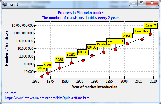![](/wiki-images/3/3d/TAChart_LogAx_Tutorial15.png)
4	4
5	5		Do you know [Moore's law](https://en.wikipedia.org/wiki/Moore's_law)? It is in front of you...
6	6
7	7		When you are reading this you are probably sitting in front of your desktop computer or have your notebook on your knees, or you are holding your smartphone in your hand. A tremendous progress of microtechnology has been happening during the last decades and is still on-going. This is due to miniaturization of electronic devices allowing to pack ever more functions onto a single silicon chip. And this is what Moore's law is about: the number of transistors on a chip has doubled approximately every two years.
8	8
9	9		In this tutorial we will take published data of an important manufacturer of microprocessors and use TAChart to plot the number of transistors versus the year of market introduction of the products. From these data we will try to confirm Moore's law.
10	10
11	11		You can find the data on the site [www.intel.com/pressroom/kits/quickreffam.htm](http://www.intel.com/pressroom/kits/quickreffam.htm) which contains a list of microprocessors, their date of market introduction, and their transistor count per chip.
12	12
13	13		When working through this example you will learn
14	14
15	15		- how to enter data at designtime
16	16		- how to create a point series with marks above each data point
17	17		- how to create a logarithmic axis
18	18		- how to fit an equation to data.
19	19
20	20		You should have some basic knowledge of how to work with TAChart; if you don't you should have a look at the [[TAChart Tutorial: Getting started\|Getting started tutorial]] of TAChart. Of course, you must be familiar with [[Lazarus]] and [[Object Pascal]]. And you should not be too afraid of math, you'll need logarithms and the exponential function.
21	21
22	22		## Preparation
23	23
24	24		### Setting up the chart
25	25
26	26		- Create a new project.
27	27		- Since we will get some long axis labels increase the size of the form to something like 540 x 320 pixels.
28	28		- Add a `TChart` component, align it to `alClient`, set its `BackColor` to `clWhite` and the `Grid.Color` of each axis to `clSilver`.
29	29		- Add a title to the x axis ("Year of market introduction") and to the y axis ("Number of transistors").
30	30		- Use the text "Progress in Microelectronics" as the chart's title.
31	31		- Set these font styles to `fsBold`.
32	32		- Show a reference for our data in the footer. Use the chart's property [[TAChart documentation\|Foot]] for that. Note that the property editor of `Foot.Text` (as well as that of `Title.Text`) allows to enter multi-lined titles.
33	33
34	34		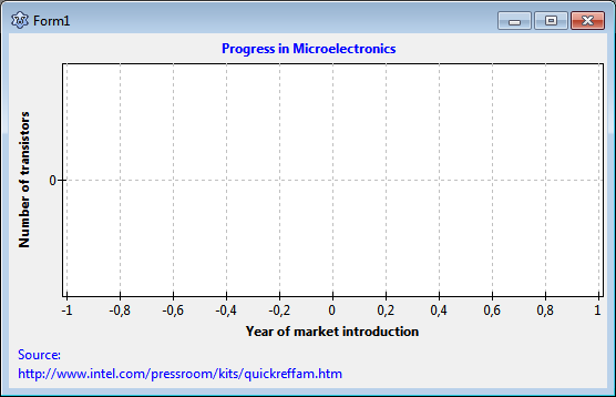![](/wiki-images/1/17/TAChart_LogAx_Tutorial1.png)
35	35
36	36		### Creating a point series
37	37
38	38		We want to draw each TDataRecord as a single data point - this is called "point series" in other charting programs. The TAChart series editor does not offer this type of series because [[TAChart documentation\|TLineSeries]] can do this as well. We only have to set its property `ShowPoints` to `true` and to turn off the connecting lines (`LineType` = `ltNone`). The symbols are determined by the property `Pointer`.
39	39
40	40		So, add a LineSeries to the form and set the properties to create a point series. Additionally, let's set the `Pointer.Brush.Color` to `clRed`, and the `Pointer.Style` to `psCircle` to draw a red circle at each data point.
41	41
42	42		## Entering data
43	43
44	44		### ListChartSource
45	45
46	46		There are many ways that data could be entered into the chart. We will use a [[TAChart documentation\|ListChartSource]] today. Usually data are loaded into this source dynamically at run-time, for example after reading a file. In our project, however, we want to enter them at design-time by means of the data point editor of the ListChartSource. This has the main advantage that all our changes that we do with the chart are displayed immediately, there is no need to compile the project. As you will see, however, there are some drawbacks as well.
47	47
48	48		The ListChartSource stores the data to be plotted in a list - that's where its name comes from. The list items are so-called `TChartDataItem` objects containing for each data point:
49	49
50	50		- the `x` and `y` coordinates,
51	51		- a `Text` to be used for data marks,
52	52		- a `Color` that overrides the SeriesColor,
53	53		- as well as a `YList` which contains additional y values which are needed in some specialized series types.
54	54
55	55		The ListChartSource is the same type of chart source that is used by many series classes internally. Having it as a separate component, however, has the big advantage that the same chart source can be used again for other series - we will need this feature later when applying the FitSeries.
56	56
57	57		![](/wiki-images/3/3b/TAChart_LogAx_Tutorial2.png) We start by adding a TListChartSource to our form. This is the second icon in the chart component palette. Connect the series to this chart source by pointing its property `Source` to the new `ListChartSource1`.
58	58
59	59		### The ListChartSource data points editor
60	60
61	61		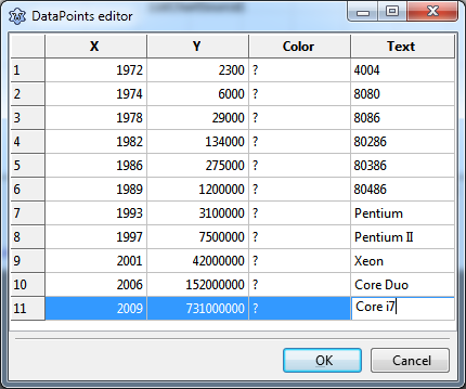![](/wiki-images/a/af/TAChart_LogAx_Tutorial16.png)
62	62
63	63		Clicking at the ellipsis button next to the property `DataPoints` opens the datapoints editor of the chart source. This is a string grid into which you can enter the data. Type in the data from the preceding image. They are an excerpt from the web site mentioned in the introduction. This site shows the time of market introduction by year and month - for simplicity, I skipped the month and rounded to the nearest calendar year. Enter the years into column X. Column Y will get the number of transistors per chip. The name of each microprocessor will go into column Text. Since we do not want to give each data point an individual color we leave the column Color alone - but, of course, you can experiment with that feature.
64	64
65	65		When you close the datapoints editor the series is automatically updated and displays the current data set. Wow!
66	66
67	67		### Displaying datapoint marks
68	68
69	69		Why don't we see the processor names that we entered in the grid? [[TAChart documentation\|Data point marks]] are turned off by default. Select the series and go to `Marks`. Look at the subproperty `Style`, it is `smsNone` which means "off". Open the dropdown list. You will see a variety of options how the data points can be labeled. Play with these settings to learn what they mean. Here we want to use `smsLabel` which displays the `Text` field of the `TChartDataItem`. In order to assign Marks.Style through source code, `uses ... TAChartUtils` shall be added.
70	70
71	71		There is also a connecting line between the label and the datapoint. Its color is white by default, that's why we cannot see it on the white background. The property name for this line is `LinkPen`. You may want to set the `LinkPen.Color` to `clGray`.
72	72
73	73		The position of the marks is OK here, but you should know that the series has a property [[TAChart documentation\|MarkPositions]] to control positioning to some degree.
74	74
75	75		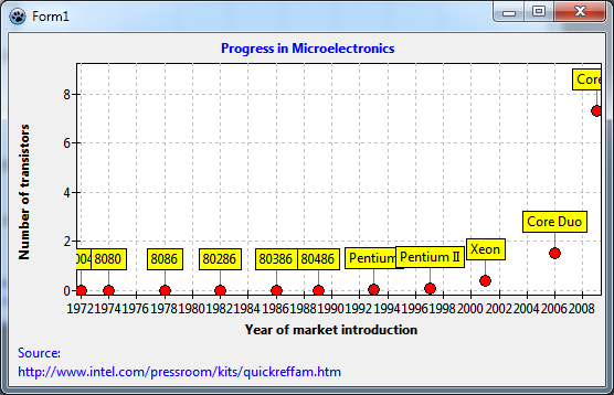![](/wiki-images/a/a4/TAChart_LogAx_Tutorial3.png)
76	76
77	77		Maybe we compile the project at this time.
78	78
79	79		There is nothing new - we saw everything already at design-time. This is a great advantage of working with the datapoints editor of a ListChartSource.
80	80
81	81		There are two things which can be improved at this stage:
82	82
83	83		- The point labels are cut off at the edges of the chart. We can fix this by increasing the chart's `Margin.Left` and `Margin.Right` to 24. [[TAChart documentation\|Margin]] defines the space surrounding the inner plot area to keep it free from data points. There is also a property [[TAChart documentation\|MarginExternal]] which surrounds the outer border of the chart and can be used to change the distance to neighboring controls.
84	84		- Since almost all data points are crowded at the bottom of the chart the plot is not very meaningful. This is why we need a logarithmic axis.
85	85
86	86		## Setting up a logarithmic axis
87	87
88	88		Plotting data on a logarithmic axis means that the logarithms of the data values are plotted, not the values directly. The y values in our diagram, for example, range between 2300 and 731 million. When we calculate the ([decadic](https://en.wikipedia.org/wiki/Common_logarithm)/log<sub>10</sub>) logarithms, the range is only between about 3.3 and 7.1 - in such a diagram the data can be distinguished much easier.
89	89
90	90		### TChartTransformations and LogarithmicAxisTransform
91	91
92	92		![](/wiki-images/3/36/TAChart_LogAx_Tutorial4.png) Calculating the logarithm can be done by TAChart automatically. The main advantage is that the original data units are drawn on the axis while the logarithms are used for plotting.
93	93
94	94		In fact, there is an entire group of components for axis transformations: [[TAChart documentation\|TChartAxisTransformations]]. An axis transformation is a function which maps "real world" data in units as displayed on the axis ("axis coordinates") to internal units that are common to all series in the same chart ("graph coordinates"). The axis coordinate of the transistor count of the 4004 processor, for example, is 2300, the graph coordinate is the logarithm of that number, i.e. log<sub>10</sub>(2300) = 3.36.
95	95
96	96		TAChart provides a variety of transforms. In addition to the logarithm transform, there is a [[TAChart documentation\|linear transform]] which allows to multiply the data by a factor and to add an offset. The [[TAChart documentation\|auto-scaling transform]] is useful when several independently scaled series have to be drawn on the same axis. The [[TAChart documentation\|user-defined transform]] allows to apply any arbitrary transformation.
97	97
98	98		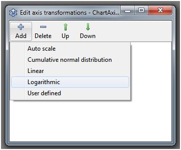![](/wiki-images/5/55/TAChart_LogAx_Tutorial5.png)
99	99
100	100		Add a `TAChartTransformations` component to the form, double-click on it (or right-click on it in the object tree and select "Edit axis transformations"), click on "Add" and select "Logarithmic". This will create a `ChartAxisTransformations1LogarithmAxisTransform1` component - what a name! Anyway, there's a high chance that you will not have to type it...
101	101
102	102		In the object inspector, you will see only a few properties - the most important one is `Base`. This is the base of the logarithm to be calculated. Change it to 10, since we want to calculate the [decadic logarithms](https://en.wikipedia.org/wiki/Common_logarithm) - this case comprises 99% of all logarithmic charts.
103	103
104	104		A side-note: it is very important that you save the project at this time. Why? You will see in a minute...
105	105
106	106		Now we must identify the axis which is to be transformed. For this purpose each axis has a property `Transformations`. In our case, the huge numbers are plotted on the y axis. So, go to the left axis and set its property `Transformations` to `ChartAxisTransformations1`.
107	107
108	108		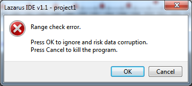![](/wiki-images/0/0d/TAChart_LogAx_Tutorial17.png)
109	109
110	110		Oh - what's that? An error message pops up reporting a range check error. Hopefully you had saved the project. If you click on Cancel Lazarus will shut down, everything will be lost. If you click on OK suddenly the chart is gone, it reappears when you click somewhere, but the faulty axis is hidden ...
111	111
112	112		Are you getting desperate?
113	113
114	114		This is the main disadvantage of working at design-time. If something goes wrong, there is no debugger, no indication of what caused the trouble. Since components are compiled into Lazarus you would have to debug the IDE. Sounds complicated...
115	115
116	116		Let's sit down and think what we did. We assigned the logarithmic transform to the y axis. The transform does not yet have any connection to the data, therefore the data are still in "real" units, their maximum is 731 million. But the transform "thinks" that the data are already in graph units (logarithms). When it calculates the axis labels in axis units it takes hundreds of millions to the power of 10! That's what causes the range check error. However, the situation is not always so dramatic; the least thing that could happen is that the data are not transformed, but the axis is.
117	117
118	118		What can we do against that? Each series has properties `AxisIndexX` and `AxisIndexY`. The transform can use this information to calculate the logarithms of the correct coordinates before the axis labels are updated. This solves our problem.
119	119
120	120		So, click on Cancel to shutdown Lazarus. Restart and reload the project. In the saved state, the transformation is not yet connected to the axis.
121	121
122	122		Now have a look at the object tree above the object inspector and you will see that the left axis has index 0. So set the series' `AxisIndexY` to this value. Although not necessary it may be a good idea to disarm also the x axis by assigning its index 1 to the `AxisIndexX` of the series - who can guarantee that we won't transform the x axis in the future?
123	123
124	124		After this is done you can set the `LeftAxis.Transformation` to `ChartTransformations1` without the range check error.
125	125
126	126		With the logarithm transform activated the data points spread nicely across the y axis range now. But what's wrong with the y axis labels? And the years on the x axis are too close and partly overlap.
127	127
128	128		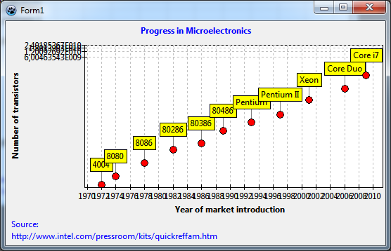![](/wiki-images/d/d0/TAChart_LogAx_Tutorial6.png)
129	129
130	130		Finding axis labels is a non-trivial task, in particular when transformations are active that heavily distort the axis intervals. Unfortunately, logarithmic axes belong to that group. Basically, there are two ways to control label positioning, an automatic and a manual way.
131	131
132	132		### Automatic finding of axis labels
133	133
134	134		For automatic label positioning, each axis has a property [[TAChart documentation\|Intervals]] which gives access to several, partly mutually excluding parameters - please see [[TAChart documentation]] for an explanation. In case of the logarithmic axis the issue is usually caused by the fact that the option `aipGraphCoordinates` is not set. This option, if set, enforces calculation of the tick intervals for the transformed data ("graph coordinates"), not the "real world" data ("axis coordinates"). So, set `aipGraphCoordinates` in the `LeftAxis.Intervals.Options`. The labels jump to more evenly distributed locations.
135	135
136	136		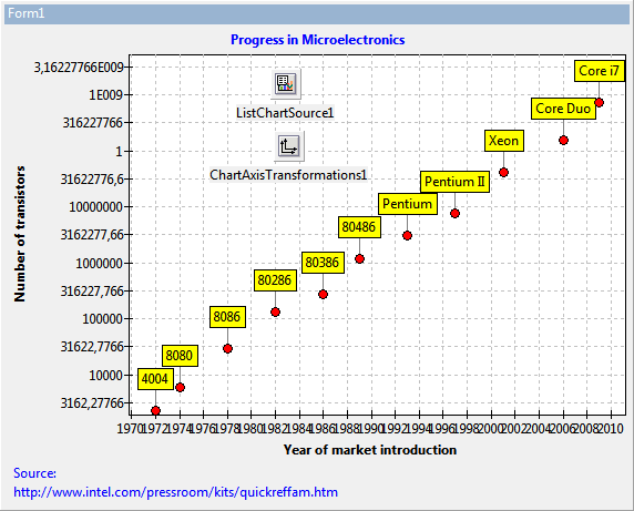![](/wiki-images/f/f1/TAChart_LogAx_Tutorial7.png)
137	137
138	138		Depending on the size of your form you may get quite nice, or not so good labels. If you resize the form you will see some "crooked" labels jump in.
139	139
140	140		You can improve the quality of label presentation in the following way:
141	141
142	142		- Increase the `Intervals.Tolerance`. This allows for varying spacing between tick marks.
143	143		- Adjust the range, in pixels, in which the label distance can vary. This is defined by the properties `Intervals.MaxLength` and `Intervals.MinLength`. The optimum value depends on the size of the chart and on the range of the data. In our example project, good labels are obtained by setting these properties to 100 and 50, respectively. Usually `Intervals.MaxLength` provides better results.
144	144
145	145		In the same way, the overlapping year labels of the x axis can be addressed. Just increase the `BottomAxis.Intervals.MaxLength` to 70.
146	146
147	147		What is left now is the "1" that appears at the y axis between "10000000" and "1E009". This is due to a bug in some FPC versions. If you have that as well, simply change the property `LeftAxis.Marks.Format`. This string is passed to the `Format` function to convert the numbers to strings. The format specifier "%0.0n" for example avoids that conversion error and, additionally, adds nice thousand separators to the labels which makes them much more readable.
148	148
149	149		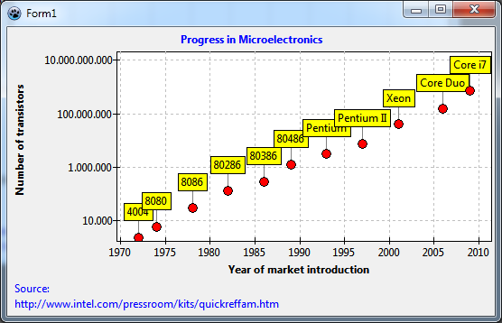![](/wiki-images/7/7e/TAChart_LogAx_Tutorial8.png)
150	150
151	151		### Manual finding of axis labels
152	152
153	153		This is the best we can do with automatic label positioning. It is not perfect because when we increase the height of the window, or zoom in, the half-decade values may appear, or the label interval may be two decades as in above figure.
154	154
155	155		If you are not happy with that you have to use manual axis label selection. For this purpose, each axis has a property `Source` which can be linked to a ListChartSource containing only the allowed axes labels. So when this chart source contains only full-decade labels there is no risk of half-decade labels or omitting every other label. On the other hand, when you zoom into the chart you may come to a point where no labels are visible any more.
156	156
157	157		Add a second ListChartSource to the form. You can use the DataPoints editor again to enter the full-decade numbers. This has the advantage that you can complete most of this project without writing a single line of code!
158	158
159	159		But you could also populate the listsource easily in the `FormCreate` event:
160	160
161	161		``` pascal
162	162		procedure TForm1.FormCreate(Sender: TObject);
163	163		const
164	164		MIN = 0;
165	165		MAX = 12;
166	166		var
167	167		i: Integer;
168	168		value: double;
169	169		begin
170	170		for i:=MIN to MAX do begin
171	171		value := Power(10, i);
172	172		ListChartSource2.Add(value, value);
173	173		end;
174	174		end;
175	175		```
176	176
177	177		This procedure adds powers of 10 in a wide enough range to the ListChartSource by means of its method `Add`.
178	178
179	179		Connect `ListChartSource1` to `LeftAxis.Marks.Source` to activate the manual labels of the ListChartSource. You should also remove all flags from the `Options` property. Otherwise automatic tick finding will still be active to some degree. If you did not use the DataPoints editor you must compile to see the effect.
180	180
181	181		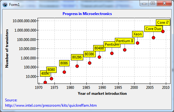![](/wiki-images/5/51/TAChart_LogAx_Tutorial9.png)
182	182
183	183		### Minor tick marks
184	184
185	185		Very often minor tick marks are placed between the major tick marks. TAChart allows to add several sets of minor ticks to each axis. We only need one here. Go to `LeftAxis` and click on the ellipsis button next to the property `Minors`. This opens the editor for `Chart1.AxisList[0].Minors`. Click on "Add" and on the "M" in the list below. Now you can adjust the parameters in the object inspector to get "good" minor ticks. If the major ticks on a logarithmic axis are at full decades then the minor ticks usually are at 2, 3, 4,..., 8, 9, and, of course, powers of 10. This can be achieved easily by turning off all `Intervals.Options` except for `aipUseCount` and setting `Intervals.Count = 9`. Of course, this makes sense only when the major labels are fixed at full decades like in the manual approach above.
186	186
187	187		Usually the plot gets too crowded by the minor grid which appears now, you should set the minor's `Grid.Visible` to `false`.
188	188
189	189		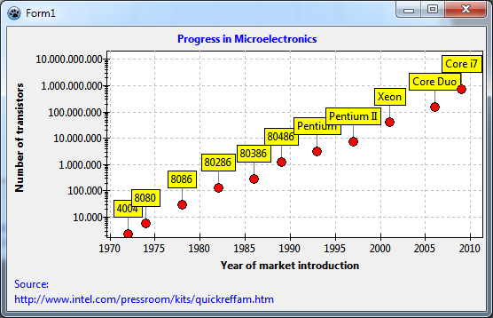![](/wiki-images/5/5c/TAChart_LogAx_Tutorial10.png)
190	190
191	191		## Fitting
192	192
193	193		Now let's look for a relation between the data, i.e. we want to find a mathematical formula which describes the dependence of transistor count on market introduction year. This is called "fitting": we select a formula with parameters and adjust the parameters such that the deviation to the data is as small as possible.
194	194
195	195		TAChart does not contain a full-fledged fitting engine. It uses the fitting routines from the FPC numerical library [[numlib]]. Therefore, TAChart cannot address all variants of fitting, but it covers the most important case, fitting of a [polynomial](https://en.wikipedia.org/wiki/Polynomial) by means of the [linear least squares technique](https://en.wikipedia.org/wiki/Least_squares). This is about the level available to Excel users when they add a "trend line" to their chart.
196	196
197	197		### TFitSeries
198	198
199	199		TAChart provides a specialized [[TAChart documentation\|TFitSeries]] for fitting. This series has a property `FitEquation` which defines the formula that is used:
200	200
201	201		- `fePolynomial`: y = b<sub>0</sub> + b<sub>1</sub>x + b<sub>2</sub>x<sup>2</sup> + … + b<sub>n</sub>x<sup>n</sup>. Specify the number of fitting parameters a<sub>i</sub> by the property `ParamCount` = n + 1.
202	202		- `feLinear`: y = a + bx -- this is a special case of the general polynomial with n = 1 and fitting parameters a and b. It is made available as a separate item because straight lines define the most important fitting conditions.
203	203		- `feExp`: y = a * e<sup>bx</sup> -- This equation can also be reduced to the polynomial case although this is not straightforward to see. But take the (natural) logarithm of this equation, and you get to ln(y) = a + bx. Now when we fit ln(y) instead of y we have the linear case again.
204	204		- `fePower`: y = a * x<sup>b</sup>. Again, this can be reduced to a linear equation by a logarithmic transformation.
205	205
206	206		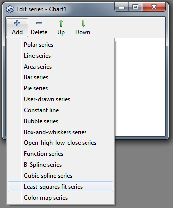![](/wiki-images/b/b5/TAChart_LogAx_Tutorial11.png)
207	207
208	208		Enough of theory. Let's add a FitSeries to the chart: double-click on the chart, and in the series editor click on "Add" and select the entry "Least squares fit series" from the dropdown list.
209	209
210	210		At first, we need to tell the fit series where it finds its data. For this purpose, we connect the series' `Source` with `ListChartSource1` as we had done with the line series. You see: the same chart source can be used for several series.
211	211
212	212		You hopefully remember the disaster above with the AxisIndex. So, set the `AxisIndexY` to the index of the left axis as we did with the line series.
213	213
214	214		Which one of the four `FitEquation` possibilities do we select? Well, the data look like lying on a straight line. So let's select `feLinear`.
215	215
216	216		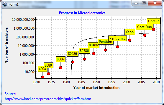![](/wiki-images/0/06/TAChart_LogAx_Tutorial12.png)
217	217
218	218		Oops... We see the black fitted curve, but it does not "fit" at all. And we wanted a straight line, but we get a twisted curve. How can this be?
219	219
220	220		The reason is the logarithmic transform that we applied to the y data. Therefore, our plot shows the logarithms, but the fit takes the "raw" data. We are effectively fitting the straight line to the data in the screenshot in the section Displaying datapoint marks where the log transform had not yet been introduced - it is clear that the line would not "fit" there. And when the fitted function is drawn the log transform distorts the straight line to the twisted curve that we see.
221	221
222	222		On the other hand, if the log data follow a straight line our fitting law is not linear, but exponential. Let's set `FitEquation` to `feExp` and try again.
223	223
224	224		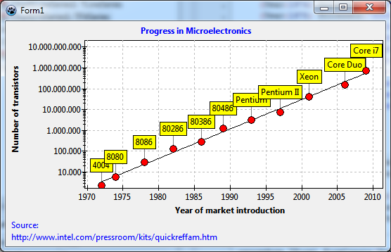![](/wiki-images/a/ac/TAChart_LogAx_Tutorial13.png)
225	225
226	226		Ah - much better!
227	227
228	228		Now we know that the exponential law, y = a * x<sup>b</sup>, is a good description of our data. But how do we get the fitting parameters a and b?
229	229
230	230		### Fit results
231	231
232	232		The fit series has a public array property `Param` which contains the fitting parameters. `a` is in `Params[0]`, and `b` is in `Params[1]`. Of course, these values are correct only when a valid fit has been performed. How do we know that? Well, the fit series provides an event `OnFitComplete` that is generated when the fit complete successfully. That's where we can evaluate the obtained fit parameters. As an example, let's display the fit results in a message along with the fit equation:
233	233
234	234		``` pascal
235	235		procedure TForm1.Chart1FitSeries1FitComplete(Sender: TObject);
236	236		begin
237	237		with Chart1FitSeries1 do
238	238		ShowMessage(Format(
239	239		'Fit result: a = %g, b = %g', [
240	240		Param[0], Param[1]
241	241		]));
242	242		end;
243	243		```
244	244
245	245		And that's what we get:
246	246
247	247		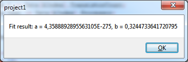![](/wiki-images/d/d1/TAChart_LogAx_Tutorial14.png)
248	248
249	249		Now we want to calculate the time T until the number of transistors on a chip is doubled. As an exercise try to show that
250	250
251		-	~~`T = ln(2) / b`~~
	251	+	```text
	252	+	T = ln(2) / b
	253	+	```
252	254
253	255		It would be nice to show the doubling time as an additional line of the chart title. For this, we modify the `OnFitComplete` event handler as follows:
254	256
255	257		``` pascal
256	258		procedure TForm1.Chart1FitSeries1FitComplete(Sender: TObject);
257	259		begin
258	260		Chart1.Title.Text.Add(Format(
259	261		'The number of transistors doubles every %.0f years',
260	262		[ln(2) / Chart1FitSeries1.Param[1]]
261	263		));
262	264		end;
263	265		```
264	266
265	267		![](/wiki-images/3/3d/TAChart_LogAx_Tutorial15.png)
266	268
267	269		Wow! This is Moore's law: "The number of transistors per chip doubles every two years"...
268	270
269	271		## Source code
270	272
271	273		### Project file
272	274
273	275		``` pascal
274	276		program project1;
275	277
276	278		{$mode objfpc}{$H+}
277	279
278	280		uses
279	281		{$IFDEF UNIX}{$IFDEF UseCThreads}
280	282		cthreads,
281	283		{$ENDIF}{$ENDIF}
282	284		Interfaces, // this includes the LCL widgetset
283	285		Forms, Unit1, tachartlazaruspkg
284	286		{ you can add units after this };
285	287
286	288		{$R *.res}
287	289
288	290		begin
289	291		//RequireDerivedFormResource := True;
290	292		Application.Initialize;
291	293		Application.CreateForm(TForm1, Form1);
292	294		Application.Run;
293	295		end.
294	296		```
295	297
296	298		### Unit1.pas
297	299
298	300		``` pascal
299	301		unit Unit1;
300	302
301	303		{$mode objfpc}{$H+}
302	304
303	305		interface
304	306
305	307		uses
306	308		Classes, SysUtils, FileUtil, TAGraph, TASeries, TASources, Forms, Controls,
307	309		Graphics, Dialogs, TACustomSource, TATransformations, TAFuncSeries;
308	310
309	311		type
310	312
311	313		{ TForm1 }
312	314
313	315		TForm1 = class(TForm)
314	316		Chart1: TChart;
315	317		Chart1FitSeries1: TFitSeries;
316	318		Chart1LineSeries1: TLineSeries;
317	319		ChartAxisTransformations1: TChartAxisTransformations;
318	320		ChartAxisTransformations1LogarithmAxisTransform1: TLogarithmAxisTransform;
319	321		ListChartSource1: TListChartSource;
320	322		ListChartSource2: TListChartSource;
321	323		procedure Chart1FitSeries1FitComplete(Sender: TObject);
322	324		procedure FormCreate(Sender: TObject);
323	325		private
324	326		{ private declarations }
325	327		public
326	328		{ public declarations }
327	329		end;
328	330
329	331		var
330	332		Form1: TForm1;
331	333
332	334		implementation
333	335
334	336		{$R *.lfm}
335	337
336	338		uses
337	339		math;
338	340
339	341		{ TForm1 }
340	342
341	343		procedure TForm1.FormCreate(Sender: TObject);
342	344		const
343	345		MIN = 0;
344	346		MAX = 12;
345	347		var
346	348		i: Integer;
347	349		value: double;
348	350		begin
349	351		for i:=MIN to MAX do begin
350	352		value := IntPower(10, i);
351	353		ListChartSource2.Add(value, value);
352	354		end;
353	355		Chart1FitSeries1.ExecFit;
354	356		end;
355	357
356	358		procedure TForm1.Chart1FitSeries1FitComplete(Sender: TObject);
357	359		begin
358	360		{
359	361		with Chart1FitSeries1 do
360	362		ShowMessage(Format(
361	363		'Fit result: a = %g, b = %g', [
362	364		Param[0], Param[1]
363	365		]));
364	366		}
365	367		Chart1.Title.Text.Add(Format(
366	368		'The number of transistors doubles every %.0f years',
367	369		[ln(2) / Chart1FitSeries1.Param[1]]
368	370		));
369	371		end;
370	372
371	373		end.
372	374		```
373	375
374	376		### Unit1.lfm
375	377
376		-	~~``` pascal~~
	378	+	``` lfm
377	379		object Form1: TForm1
378	380		Left = 244
379	381		Height = 356
380	382		Top = 193
381	383		Width = 552
382	384		Caption = 'Form1'
383	385		ClientHeight = 356
384	386		ClientWidth = 552
385	387		OnCreate = FormCreate
386	388		LCLVersion = '1.1'
387	389		object Chart1: TChart
388	390		Left = 0
389	391		Height = 356
390	392		Top = 0
391	393		Width = 552
392	394		AxisList = <
393	395		item
394	396		Grid.Color = clSilver
395	397		Marks.Format = '%0:.0n'
396	398		Marks.Source = ListChartSource2
397	399		Marks.Style = smsCustom
398	400		Minors = <
399	401		item
400	402		Grid.Visible = False
401	403		Intervals.Count = 9
402	404		Intervals.MinLength = 5
403	405		Intervals.Options = [aipUseCount]
404	406		end>
405	407		Title.LabelFont.Orientation = 900
406	408		Title.LabelFont.Style = [fsBold]
407	409		Title.Visible = True
408	410		Title.Caption = 'Number of transistors'
409	411		Transformations = ChartAxisTransformations1
410	412		end
411	413		item
412	414		Grid.Color = clSilver
413	415		Intervals.MaxLength = 60
414	416		Alignment = calBottom
415	417		Minors = <>
416	418		Title.LabelFont.Style = [fsBold]
417	419		Title.Visible = True
418	420		Title.Caption = 'Year of market introduction'
419	421		end>
420	422		BackColor = clWhite
421	423		Foot.Alignment = taLeftJustify
422	424		Foot.Brush.Color = clBtnFace
423	425		Foot.Font.Color = clBlue
424	426		Foot.Text.Strings = (
425	427		'Source:'
426	428		'http://www.intel.com/pressroom/kits/quickreffam.htm'
427	429		)
428	430		Foot.Visible = True
429	431		Margins.Left = 24
430	432		Margins.Right = 24
431	433		Title.Brush.Color = clBtnFace
432	434		Title.Font.Color = clBlue
433	435		Title.Font.Style = [fsBold]
434	436		Title.Text.Strings = (
435	437		'Progress in Microelectronics'
436	438		)
437	439		Title.Visible = True
438	440		Align = alClient
439	441		ParentColor = False
440	442		object Chart1LineSeries1: TLineSeries
441	443		Marks.Format = '%2:s'
442	444		Marks.LinkPen.Color = clGray
443	445		Marks.Style = smsLabel
444	446		AxisIndexY = 0
445	447		LineType = ltNone
446	448		Pointer.Brush.Color = clRed
447	449		Pointer.Style = psCircle
448	450		ShowPoints = True
449	451		Source = ListChartSource1
450	452		end
451	453		object Chart1FitSeries1: TFitSeries
452	454		AxisIndexX = 1
453	455		AxisIndexY = 0
454	456		FitEquation = feExp
455	457		OnFitComplete = Chart1FitSeries1FitComplete
456	458		ParamCount = 2
457	459		Source = ListChartSource1
458	460		end
459	461		end
460	462		object ListChartSource1: TListChartSource
461	463		DataPoints.Strings = (
462	464		'1972\|2300\|?\|4004'
463	465		'1974\|6000\|?\|8080'
464	466		'1978\|29000\|?\|8086'
465	467		'1982\|134000\|?\|80286'
466	468		'1986\|275000\|?\|80386'
467	469		'1989\|1200000\|?\|80486'
468	470		'1993\|3100000\|?\|Pentium'
469	471		'1997\|7500000\|?\|Pentium II'
470	472		'2001\|42000000\|?\|Xeon'
471	473		'2006\|152000000\|?\|Core Duo'
472	474		'2009\|731000000\|?\|Core i7'
473	475		)
474	476		left = 240
475	477		top = 40
476	478		end
477	479		object ChartAxisTransformations1: TChartAxisTransformations
478	480		left = 243
479	481		top = 96
480	482		object ChartAxisTransformations1LogarithmAxisTransform1: TLogarithmAxisTransform
481	483		Base = 10
482	484		end
483	485		end
484	486		object ListChartSource2: TListChartSource
485	487		left = 243
486	488		top = 176
487	489		end
488	490		end
489	491		```
490	492
491	493		---
492	494		From the Free Pascal wiki, page "TAChart Tutorial: ListChartSource, Logarithmic Axis, Fitting", as it stood on 2020-02-29 after a change by Trev, out of the wiki's dump of 2024-05-26. Copyright stays with the author who wrote it, according to the old wiki's [[Licensing]] page. If you have concerns about this material, [message the admin](/wiki-contact).

Back to history