TAChart Tutorial: ListChartSource, Logarithmic Axis, Fitting/fi: what changed

Revision 1 to 2. Removed lines have a minus sign; added lines have a plus sign.

Old	New		Line
1	1		## Johdanto
2	2
3	3		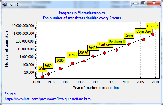![](/wiki-images/3/3d/TAChart_LogAx_Tutorial15.png)
4	4
5	5		Tiedätkö mikä on [Mooren laki](http://fi.wikipedia.org/wiki/Mooren_laki)? Siihen tutustutaan tässä esimerkissä.
6	6
7	7		Lukiessasi tätä olet todennäköisesti pöytätietokoneen, kannettavan tai älypuhelimen ääressä. Valtava edistyminen mikrotietokoneteknologiassa on tapahtunut viimeisten vuosikymmenten aikana ja on edelleen käynnissä. Tämä pienentäminen elektronissa laitteissa mahdollistaa pakata yhä enemmän toimintoja yhdelle piisirulle. Ja mitä Mooren laki on: transistoreiden määrä sirulla on kaksinkertaistunut noin kahden vuoden välein.
8	8
9	9		Tässä opetusohjelmassa otamme datan mikroprosessorien valmistajan julkaistuista tiedoista ja käytetään TAChart piirtämään transistoreihen määrää piirillä eri vuosina markkinoille tulleista tuotteista. Näiden tietojen avulla yritämme vahvistaa Mooren lain.
10	10
11	11		Tässä käytettävä data löytyy sivustolta [www.intel.com/pressroom/kits/quickreffam.htm](http://www.intel.com/pressroom/kits/quickreffam.htm) joka sisältää luettelon mikroprosessoreista, ajankohdista niiden tuomisista markkinoille ja niiden sisältämä transistorin määrä per piiri.
12	12
13	13		Tässä esimerkissä opitaan
14	14
15	15		- miten syötetään dataa suunnitteluaikana
16	16		- miten luodaan pistekuvaaja jossa nimiteksti kullakin datapisteellä
17	17		- miten luodaan logaritminen akseli
18	18		- miten sovittaa yhtälö tietoihin.
19	19
20	20		Sinulla pitäisi olla joitakin perustietoja miten työskennellä TAChart-komponentin kanssa jos ei ole niin katso [[TAChart Tutorial: Getting started/fi\|TAChart:n aloitusopas]]. Tietenkin, sinun on tunnettava [[Lazarus]] ja [[Object Pascal]] . Eikä myöskään saisi pelätä matematiikkaa (käytössä logaritmit ja eksponenttifunktio).
21	21
22	22		## Valmistautuminen
23	23
24	24		### Kaavion tekeminen
25	25
26	26		- Luo uusi projekti.
27	27		- Koska laitamme joitakin pitkiä otsikoita akselille niin kasvata lomakkeen kokoa vähintään 540 x 320 pikseliin.
28	28		- Lisää `TChart` komponentti, laita komponenttimuokkaimessa sen align arvoon `alClient`, Aseta sen `BackColor` arvoksi `clWhite` ja `Grid.Color` molemmille akselille arvoon `clSilver`.
29	29		- Lisää otsikoksi x-akselille "Year of market introduction" (tai suomenkielisenä "Markkinoilletulo vuosi") ja y-akselille "Number of transistors" (Transistorien määrä).
30	30		- Lisää teksti "Progress in Microelectronics" (tai "Mikroelektroniikan edistys") koko kaavion otsikoksi.
31	31		- Aseta näiden fontin tyyliksi `fsBold`.
32	32		- Näytä viitteenä datan lähde alatunnisteessa. Käytä kaavion ominaisuutta [[TAChart documentation\|Foot]] siinä. Huomaa, että omaisuus `Foot.Text` (samoin kuin `Title.Text` ) voi syöttää usean rivin otsikon.
33	33
34	34		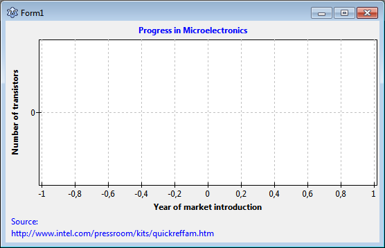![](/wiki-images/1/17/TAChart_LogAx_Tutorial1.png)
35	35
36	36		### Luodaan pistekuvaaja
37	37
38	38		Kun halutaan piirtää kullekin datatietueelle yksi piste - tätä usein kutsutaan pistekuvaajaksi muissa kaavio-ohjelmissa. TAChart kuvajaajissa ei ole tälläistä kuvaajaa koska [[TAChart documentation\|TLineSeries]] voi tehdä tämän yhtähyvin. Laittamalla sen ominaisuus `ShowPoints` arvoon `true` ja poistamalla yhdistävät viivat (`LineType` = `ltNone`). Näytettävat datapisteet kuvataan ominaisuudessa `Pointer`.
39	39
40	40		Niin lisätään viivakuvaaja (LineSeries) ja asetetaan sen ominaisuudet niin että siitä tulee pistekuvaaja. Lisäksi asetetaan `Pointer.Brush.Color` arvoon `clRed` ja `Pointer.Style` arvoon `psCircle` tämä asettaa näyttämään kunkin datapisteen punaiselta ympyrältä.
41	41
42	42		## Syötetään data
43	43
44	44		### ListChartSource
45	45
46	46		On monia tapoja, joilla tietoja voidaan syöttää kaavioon. Nyt tässä käytetään [[TAChart documentation\|ListChartSource]]:a. Yleensä tiedot ladataan tähän dynaamisesti ajon aikana, esimerkiksi lukemalla tiedot tiedostosta. Tässä projektissa kuitenkin data syötetään suunnitteluaikana käyttämällä datapisteen päätoimittaja ListChartSource. Tämän suurin etu on että kaikki muutokset, jotka tehdään kaavioon näytetään heti, ei tarvitse edes kääntää projektia. Kuten , on kuitenkin olemassa joitakin haittoja samoin.
47	47
48	48		ListChartSource tallentaa piirrettävän datan luetteloon - siitähän sen englanninkielinen nimi tulee. Luettelossa olevia kohteita kutsutaan `TChartDataItem` :ksi. Se sisältää datapisteen tietoja:
49	49
50	50		- `x` ja `y` koordinaatit,
51	51		- `Text` jota käytetään datan merkintään
52	52		- `Color` eli väri-tieto joka ylikirjoittaa kuvaajan oletusvärin (SeriesColor)
53	53		- `YList` joka sisältää lisää y:n arvoja joita tarvitaan joissakin erikoistapauksissa.
54	54
55	55		ListChartSource on samantyyppinen kaavion lähde, joka on käytössä monien kuvaajien luokkien sisällä. Kun se on erillinen komponentti on siitä kuitenkin etua, että samaa kaavion lähdettä voidaan käyttää uudelleen muissa kuvaajissa - tarvitsemme tätä ominaisuutta myöhemmin sovellettaessa FitSeries.
56	56
57	57		![](/wiki-images/3/3b/TAChart_LogAx_Tutorial2.png) Lisäämällä TListChartSource lomakkeelle. Tämä löytyy toisena kuvakeena chart-komponenttipaletilta. Kytke kuvaaja osoittamaan tähän lähteeseen asettamalla ominaisuus `Source` uuteen arvoon `ListChartSource1`.
58	58
59	59		### ListChartSource datapisteiden muokkain
60	60
61	61		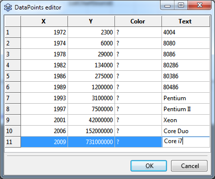![](/wiki-images/a/af/TAChart_LogAx_Tutorial16.png)
62	62
63	63		Klikkaamalla kolmeapistepainiketta ominaisuudessa `DataPoints` avautuu datapisteiden muokkain. Tämä on ruudukko, johon syötetään tiedot. Kirjoita tiedot yllä olevasta kuvasta. Ne ovat otettu verkkosivuilta joka mainitaan johdannossa. Tämä sivusto näyttää markkinoille tulon ajan vuosittain ja kuukausittain - yksinkertaisuuden vuoksi ohitetaan kuukausi ja pyöristetään se lähimpään kalenterivuoteen. Anna vuosi sarakkeeseen X. Sarake Y saa transistorien määrä per piiri. Jokaisen mikroprosessorin nimi siirtyy sarakkeeseen Teksti. Koska ei anneta yksittäisen datapisteen väriä ohitetaan sarake Väri - mutta tietenkin sitä ominaisuutta voi kokeilla muuttaa.
64	64
65	65		Kun datapisteiden muokkain suljetaan niin sarja päivitetään automaattisesti ja näkyvissä on päivitetty tietojoukko. Vau!
66	66
67	67		### Näytetään datapisteen nimi
68	68
69	69		Miksi emme näe prosessorien nimiä jotka asetettiin ruudukossa? [[TAChart documentation\|Datapisteen nimi]] on oletuksena pois päältä. Valitse kuvaaja ja siirry kohtaan `Marks` . Katso aliominaisuutta `Style` , se on `smsNone` joka tarkoittaa "off" eli poispäältä. Avaa kyseisen kohdan pudotusvalikko. Näet erilaisia vaihtoehtoja kuinka datapisteiden nimi voidaan merkitä. Testaa eri asetuksia. Jo suunnitteluaikana nähdään mitä ne tarkoittavat. Ota lopuksi käyttöön `smsLabel` joka näyttää tekstin.
70	70
71	71		On myös yhdistävä viiva nimen ja datapisteen välillä. Sen väri on oletuksena valkoinen, siksi sitä ei nähdä valkoisella taustalla. Tämän viivan ominaisuuksia muutetaan `LinkPen` kohdan alla. Aseta `LinkPen.Color` arvoon `clGray` .
72	72
73	73		Näiden nimien paikkaa pystyy jossain määrin muuttamaan [[TAChart documentation\|MarkPositions]] ominaisuudessa.
74	74
75	75		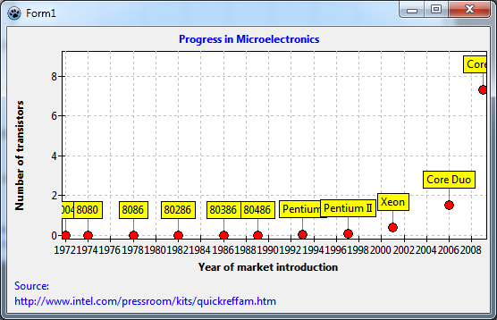![](/wiki-images/a/a4/TAChart_LogAx_Tutorial3.png)
76	76
77	77		Jos ohjelma käännetään nyt niin mitään uutta ei tule verrattuna suunnitteluaikaiseen näkymään. Tämä on suuri etu kun työskentelee ListChartSource:n datapisteiden muokkaimella.
78	78
79	79		On kaksi asiaa, joita voidaan parantaa tässä vaiheessa:
80	80
81	81		- Kaavion reunoilla datapisteiden nimet leikkautuvat pois. Sitä ei voi korjata lisäämällä kaavion `Margin.Left` ja `Margin.Right` arvoksi 24. Koska [[TAChart documentation\|Margin]] määrittää ympäröivän tilan sisemmällä alueella pitää sen vapaana datapisteistä. On myös ominaisuus [[TAChart documentation\|MarginExternal]] joka ympäröi kaavion ulompaa aluetta ja sillä voidaan muuttaa etäisyyttä naapurikontrolleihin.
82	82		- Koska lähes kaikki datapisteet ovat kaavion alareunassa niin se ei ole kovin mielekästä. Tämän vuoksi tarvitsemme logaritmistä akselia.
83	83
84	84		## Otetaan logaritminen akseli käyttöön
85	85
86	86		Datan näyttäminen logaritmisella akselilla tarkoittaa, että logaritmit data-arvot on piirretty, ei arvoja suoraan. Kaaviossa Y: n arvot vaihtelevat välillä 2300 ja 731 miljoonaa. Kun lasketaan ([decadic](https://en.wikipedia.org/wiki/Common_logarithm)/log<sub>10</sub>) logaritmit, alue on vain noin 3,3 ja 7,1 - tällaisessa kaaviossa tämä data voidaan erottaa paljon helpommin toisistaan.
87	87
88	88		### TChartTransformations and LogarithmicAxisTransform
89	89
90	90		![](/wiki-images/3/36/TAChart_LogAx_Tutorial4.png) Calculating the logarithm can be done by TAChart automatically. The main advantage is that the original data units are drawn on the axis while the logarithms are used for plotting.
91	91
92	92		In fact, there is an entire group of components for axis transformations: [[TAChart documentation\|TChartAxisTransformations]]. An axis transformation is a function which maps "real world" data in units as displayed on the axis ("axis coordinates") to internal units that are common to all series in the same chart ("graph coordinates"). The axis coordinate of the transistor count of the 4004 processor, for example, is 2300, the graph coordinate is the logarithm of that number, i.e. log<sub>10</sub>(2300) = 3.36.
93	93
94	94		TAChart provides a variety of transforms. In addition to the logarithm transform, there is a [[TAChart documentation\|linear transform]] which allows to multiply the data by a factor and to add an offset. The [[TAChart documentation\|auto-scaling transform]] is useful when several independently scaled series have to be drawn on the same axis. The [[TAChart documentation\|user-defined transform]] allows to apply any arbitrary transformation.
95	95
96	96		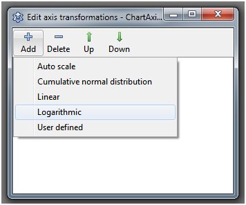![](/wiki-images/5/55/TAChart_LogAx_Tutorial5.png)
97	97
98	98		Add a `TAChartTransformations` component to the form, double-click on it (or right-click on it in the object tree and select "Edit axis transformations"), click on "Add" and select "Logarithmic". This will create a `ChartAxisTransformations1LogarithmAxisTransform1` component - what a name! Anyway, there's a high chance that you will not have to type it...
99	99
100	100		In the object inspector, you will see only a few properties - the most important one is `Base`. This is the base of the logarithm to be calculated. Change it to 10, since we want to calculate the [decadic logarithms](https://en.wikipedia.org/wiki/Common_logarithm) - this case comprises 99% of all logarithmic charts.
101	101
102	102		A side-note: it is very important that you save the project at this time. Why? You will see in a minute...
103	103
104	104		Now we must identify the axis which is to be transformed. For this purpose each axis has a property `Transformations`. In our case, the huge numbers are plotted on the y axis. So, go to the left axis and set its property `Transformations` to `ChartAxisTransformations1`.
105	105
106	106		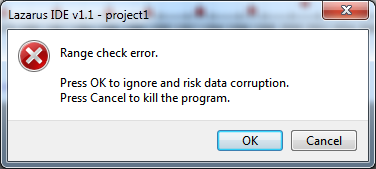![](/wiki-images/0/0d/TAChart_LogAx_Tutorial17.png)
107	107
108	108		Oh - what's that? An error message pops up reporting a range check error. Hopefully you had saved the project. If you click on Cancel Lazarus will shut down, everything will be lost. If you click on OK suddenly the chart is gone, it reappears when you click somewhere, but the faulty axis is hidden ...
109	109
110	110		Are you getting desperate?
111	111
112	112		This is the main disadvantage of working at design-time. If something goes wrong, there is no debugger, no indication of what caused the trouble. Since components are compiled into Lazarus you would have to debug the IDE. Sounds complicated...
113	113
114	114		Let's sit down and think what we did. We assigned the logarithmic transform to the y axis. The transform does not yet have any connection to the data, therefore the data are still in "real" units, their maximum is 731 million. But the transform "thinks" that the data are already in graph units (logarithms). When it calculates the axis labels in axis units it takes hundreds of millions to the power of 10! That's what causes the range check error. However, the situation is not always so dramatic; the least thing that could happen is that the data are not transformed, but the axis is.
115	115
116	116		What can we do against that? Each series has properties `AxisIndexX` and `AxisIndexY`. The transform can use this information to calculate the logarithms of the correct coordinates before the axis labels are updated. This solves our problem.
117	117
118	118		So, click on Cancel to shutdown Lazarus. Restart and reload the project. In the saved state, the transformation is not yet connected to the axis.
119	119
120	120		Now have a look at the object tree above the object inspector and you will see that the left axis has index 0. So set the series' `AxisIndexY` to this value. Although not necessary it may be a good idea to disarm also the x axis by assigning its index 1 to the `AxisIndexX` of the series - who can guarantee that we won't transform the x axis in the future?
121	121
122	122		After this is done you can set the `LeftAxis.Transformation` to `ChartTransformations1` without the range check error.
123	123
124	124		With the logarithm transform activated the data points spread nicely across the y axis range now. But what's wrong with the y axis labels? And the years on the x axis are too close and partly overlap.
125	125
126	126		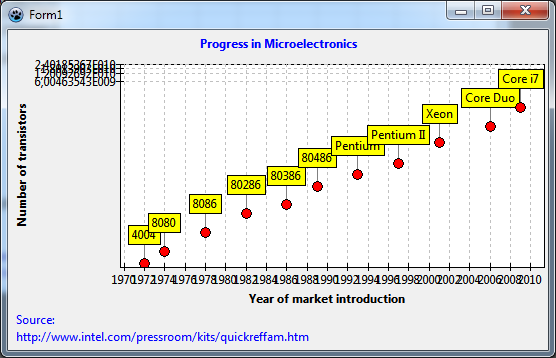![](/wiki-images/d/d0/TAChart_LogAx_Tutorial6.png)
127	127
128	128		Finding axis labels is a non-trivial task, in particular when transformations are active that heavily distort the axis intervals. Unfortunately, logarithmic axes belong to that group. Basically, there are two ways to control label positioning, an automatic and a manual way.
129	129
130	130		### Automatic finding of axis labels
131	131
132	132		For automatic label positioning, each axis has a property [[TAChart documentation\|Intervals]] which gives access to several, partly mutually excluding parameters - please see [[TAChart documentation]] for an explanation. In case of the logarithmic axis the issue is usually caused by the fact that the option `aipGraphCoordinates` is not set. This option, if set, enforces calculation of the tick intervals for the transformed data ("graph coordinates"), not the "real world" data ("axis coordinates"). So, set `aipGraphCoordinates` in the `LeftAxis.Intervals.Options`. The labels jump to more evenly distributed locations.
133	133
134	134		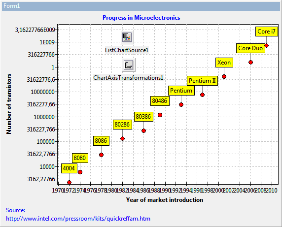![](/wiki-images/f/f1/TAChart_LogAx_Tutorial7.png)
135	135
136	136		Depending on the size of your form you may get quite nice, or not so good labels. If you resize the form you will see some "crooked" labels jump in.
137	137
138	138		You can improve the quality of label presentation in the following way:
139	139
140	140		- Moderately increase the `Intervals.Tolerance` to something like 5.
141	141		- Adjust the range in which the label distance can vary. This is defined by the properties `Intervals.MaxLength` and `Intervals.MinLength`. The optimum value depends on the size of the chart and on the range of the data. In our example project, good labels are obtained by setting these properties to 100 and 50, respectively.
142	142
143	143		In the same way, the overlapping year labels of the x axis can be addressed. Just increase the `BottomAxis.Intervals.MaxLength` to 70.
144	144
145	145		What is left now is the "1" that appears at the y axis between "10000000" and "1E009". This is due to a bug in some FPC versions. If you have that as well, simply change the property `LeftAxis.Marks.Format`. This string is passed to the `Format` function to convert the numbers to strings. The format specifier "%0.0n" for example avoids that conversion error and, additionally, adds nice thousand separators to the labels which makes them much more readable.
146	146
147	147		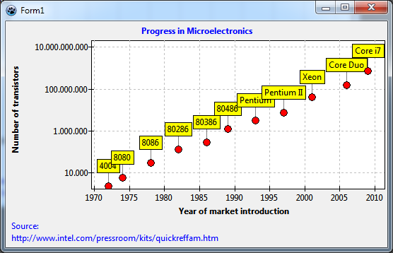![](/wiki-images/7/7e/TAChart_LogAx_Tutorial8.png)
148	148
149	149		### Manual finding of axis labels
150	150
151	151		This is the best we can do with automatic label positioning. It is not perfect because when we increase the height of the window, or zoom in, the half-decade values may appear, or the label interval may be two decades as in above figure.
152	152
153	153		If you are not happy with that you have to use manual axis label selection. For this purpose, each axis has a property `Source` which can be linked to a ListChartSource containing only the allowed axes labels. So when this chart source contains only full-decade labels there is no risk of half-decade labels or omitting every other label. On the other hand, when you zoom into the chart you may come to a point where no labels are visible any more.
154	154
155	155		Add a second ListChartSource to the form. You can use the DataPoints editor again to enter the full-decade numbers. This has the advantage that you can complete most of this project without writing a single line of code!
156	156
157	157		But you could also populate the listsource easily in the `FormCreate` event:
158	158
159	159		``` pascal
160	160		procedure TForm1.FormCreate(Sender: TObject);
161	161		const
162	162		MIN = 0;
163	163		MAX = 12;
164	164		var
165	165		i: Integer;
166	166		value: double;
167	167		begin
168	168		for i:=MIN to MAX do begin
169	169		value := Power(10, i);
170	170		ListChartSource2.Add(value, value);
171	171		end;
172	172		end;
173	173		```
174	174
175	175		This procedure adds powers of 10 in a wide enough range to the ListChartSource by means of its method `Add`.
176	176
177	177		Connect `ListChartSource1` to `LeftAxis.Marks.Source` to activate the manual labels of the ListChartSource. You should also remove all flags from the `Options` property. Otherwise automatic tick finding will still be active to some degree. If you did not use the DataPoints editor you must compile to see the effect.
178	178
179	179		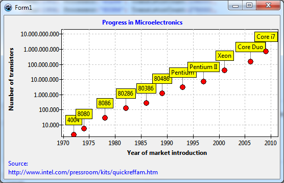![](/wiki-images/5/51/TAChart_LogAx_Tutorial9.png)
180	180
181	181		### Minor tick marks
182	182
183	183		Very often minor tick marks are placed between the major tick marks. TAChart allows to add several sets of minor ticks to each axis. We only need one here. Go to `LeftAxis` and click on the ellipsis button next to the property `Minors`. This opens the editor for `Chart1.AxisList[0].Minors`. Click on "Add" and on the "M" in the list below. Now you can adjust the parameters in the object inspector to get "good" minor ticks. If the major ticks on a logarithmic axis are at full decades then the minor ticks usually are at 2, 3, 4,..., 8, 9, and, of course, powers of 10. This can be achieved easily by turning off all `Intervals.Options` except for `aipUseCount` and setting `Intervals.Count = 9`. Of course, this makes sense only when the major labels are fixed at full decades like in the manual approach above.
184	184
185	185		Usually the plot gets too crowded by the minor grid which appears now, you should set the minor's `Grid.Visible` to `false`.
186	186
187	187		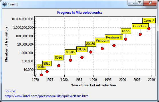![](/wiki-images/5/5c/TAChart_LogAx_Tutorial10.png)
188	188
189	189		## Fitting
190	190
191	191		Now let's look for a relation between the data, i.e. we want to find a mathematical formula which describes the dependence of transistor count on market introduction year. This is called "fitting": we select a formula with parameters and adjust the parameters such that the deviation to the data is as small as possible.
192	192
193	193		TAChart does not contain a full-fledged fitting engine. It uses the fitting routines from the FPC numerical library [[numlib]]. Therefore, TAChart cannot address all variants of fitting, but it covers the most important case, fitting of a [polynomial](https://en.wikipedia.org/wiki/Polynomial) by means of the [linear least squares technique](https://en.wikipedia.org/wiki/Least_squares). This is about the level available to Excel users when they add a "trend line" to their chart.
194	194
195	195		### TFitSeries
196	196
197	197		TAChart provides a specialized [[TAChart documentation\|TFitSeries]] for fitting. This series has a property `FitEquation` which defines the formula that is used:
198	198
199	199		- `fePolynomial`: y = b<sub>0</sub> + b<sub>1</sub>x + b<sub>2</sub>x<sup>2</sup> + … + b<sub>n</sub>x<sup>n</sup>. Specify the number of fitting parameters a<sub>i</sub> by the property `ParamCount` = n + 1.
200	200		- `feLinear`: y = a + bx -- this is a special case of the general polynomial with n = 1 and fitting parameters a and b. It is made available as a separate item because straight lines define the most important fitting conditions.
201	201		- `feExp`: y = a * e<sup>bx</sup> -- This equation can also be reduced to the polynomial case although this is not straightforward to see. But take the (natural) logarithm of this equation, and you get to ln(y) = a + bx. Now when we fit ln(y) instead of y we have the linear case again.
202	202		- `fePower`: y = a * x<sup>b</sup>. Again, this can be reduced to a linear equation by a logarithmic transformation.
203	203
204	204		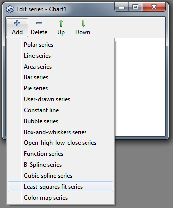![](/wiki-images/b/b5/TAChart_LogAx_Tutorial11.png)
205	205
206	206		Enough of theory. Let's add a FitSeries to the chart: double-click on the chart, and in the series editor click on "Add" and select the entry "Least squares fit series" from the dropdown list.
207	207
208	208		At first, we need to tell the fit series where it finds its data. For this purpose, we connect the series' `Source` with `ListChartSource1` as we had done with the line series. You see: the same chart source can be used for several series.
209	209
210	210		You hopefully remember the disaster above with the AxisIndex. So, set the `AxisIndexY` to the index of the left axis as we did with the line series.
211	211
212	212		Which one of the four `FitEquation` possibilities do we select? Well, the data look like lying on a straight line. So let's select `feLinear`.
213	213
214	214		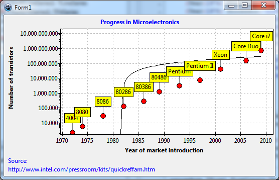![](/wiki-images/0/06/TAChart_LogAx_Tutorial12.png)
215	215
216	216		Oops... We see the black fitted curve, but it does not "fit" at all. And we wanted a straight line, but we get a twisted curve. How can this be?
217	217
218	218		The reason is the logarithmic transform that we applied to the y data. Therefore, our plot shows the logarithms, but the fit takes the "raw" data. We are effectively fitting the straight line to the data in the screenshot in the section Displaying datapoint marks where the log transform had not yet been introduced - it is clear that the line would not "fit" there. And when the fitted function is drawn the log transform distorts the straight line to the twisted curve that we see.
219	219
220	220		On the other hand, if the log data follow a straight line our fitting law is not linear, but exponential. Let's set `FitEquation` to `feExp` and try again.
221	221
222	222		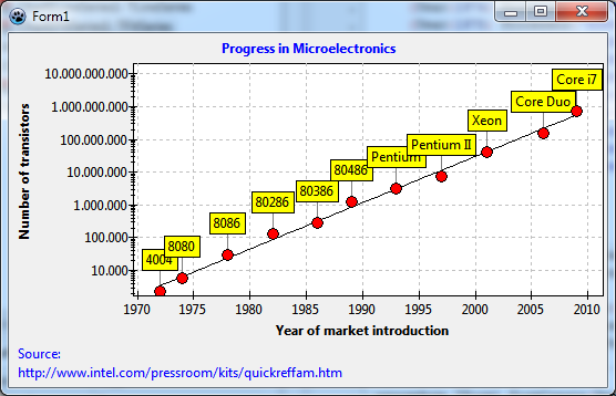![](/wiki-images/a/ac/TAChart_LogAx_Tutorial13.png)
223	223
224	224		Ah - much better!
225	225
226	226		Now we know that the exponential law, y = a * x<sup>b</sup>, is a good description of our data. But how do we get the fitting parameters a and b?
227	227
228	228		### Fit results
229	229
230	230		The fit series has a public array property `Param` which contains the fitting parameters. `a` is in `Params[0]`, and `b` is in `Params[1]`. Of course, these values are correct only when a valid fit has been performed. How do we know that? Well, the fit series provides an event `OnFitComplete` that is generated when the fit complete successfully. That's where we can evaluate the obtained fit parameters. As an example, let's display the fit results in a message along with the fit equation:
231	231
232	232		``` pascal
233	233		procedure TForm1.Chart1FitSeries1FitComplete(Sender: TObject);
234	234		begin
235	235		with Chart1FitSeries1 do
236	236		ShowMessage(Format(
237	237		'Fit result: a = %g, b = %g', [
238	238		Param[0], Param[1]
239	239		]));
240	240		end;
241	241		```
242	242
243	243		And that's what we get:
244	244
245	245		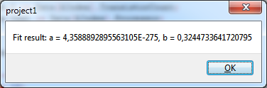![](/wiki-images/d/d1/TAChart_LogAx_Tutorial14.png)
246	246
247	247		Now we want to calculate the time T until the number of transistors on a chip is doubled. As an exercise try to show that
248	248
249		-	~~`T = ln(2) / b`~~
	249	+	```text
	250	+	T = ln(2) / b
	251	+	```
250	252
251	253		It would be nice to show the doubling time as an additional line of the chart title. For this, we modify the `OnFitComplete` event handler as follows:
252	254
253	255		``` pascal
254	256		procedure TForm1.Chart1FitSeries1FitComplete(Sender: TObject);
255	257		begin
256	258		Chart1.Title.Text.Add(Format(
257	259		'The number of transistors doubles every %.0f years',
258	260		[ln(2) / Chart1FitSeries1.Param[1]]
259	261		));
260	262		end;
261	263		```
262	264
263	265		![](/wiki-images/3/3d/TAChart_LogAx_Tutorial15.png)
264	266
265	267		Vau! Tämä on Mooren laki: "Transistoreiden määrä per siru kaksinkertaistuu kahden vuoden välein" ...
266	268
267	269		## Lähdekoodi
268	270
269	271		### Project file
270	272
271	273		``` pascal
272	274		program project1;
273	275
274	276		{$mode objfpc}{$H+}
275	277
276	278		uses
277	279		{$IFDEF UNIX}{$IFDEF UseCThreads}
278	280		cthreads,
279	281		{$ENDIF}{$ENDIF}
280	282		Interfaces, // this includes the LCL widgetset
281	283		Forms, Unit1, tachartlazaruspkg
282	284		{ you can add units after this };
283	285
284	286		{$R *.res}
285	287
286	288		begin
287	289		//RequireDerivedFormResource := True;
288	290		Application.Initialize;
289	291		Application.CreateForm(TForm1, Form1);
290	292		Application.Run;
291	293		end.
292	294		```
293	295
294	296		### Unit1.pas
295	297
296	298		``` pascal
297	299		unit Unit1;
298	300
299	301		{$mode objfpc}{$H+}
300	302
301	303		interface
302	304
303	305		uses
304	306		Classes, SysUtils, FileUtil, TAGraph, TASeries, TASources, Forms, Controls,
305	307		Graphics, Dialogs, TACustomSource, TATransformations, TAFuncSeries;
306	308
307	309		type
308	310
309	311		{ TForm1 }
310	312
311	313		TForm1 = class(TForm)
312	314		Chart1: TChart;
313	315		Chart1FitSeries1: TFitSeries;
314	316		Chart1LineSeries1: TLineSeries;
315	317		ChartAxisTransformations1: TChartAxisTransformations;
316	318		ChartAxisTransformations1LogarithmAxisTransform1: TLogarithmAxisTransform;
317	319		ListChartSource1: TListChartSource;
318	320		ListChartSource2: TListChartSource;
319	321		procedure Chart1FitSeries1FitComplete(Sender: TObject);
320	322		procedure FormCreate(Sender: TObject);
321	323		private
322	324		{ private declarations }
323	325		public
324	326		{ public declarations }
325	327		end;
326	328
327	329		var
328	330		Form1: TForm1;
329	331
330	332		implementation
331	333
332	334		{$R *.lfm}
333	335
334	336		uses
335	337		math;
336	338
337	339		{ TForm1 }
338	340
339	341		procedure TForm1.FormCreate(Sender: TObject);
340	342		const
341	343		MIN = 0;
342	344		MAX = 12;
343	345		var
344	346		i: Integer;
345	347		value: double;
346	348		begin
347	349		for i:=MIN to MAX do begin
348	350		value := IntPower(10, i);
349	351		ListChartSource2.Add(value, value);
350	352		end;
351	353		Chart1FitSeries1.ExecFit;
352	354		end;
353	355
354	356		procedure TForm1.Chart1FitSeries1FitComplete(Sender: TObject);
355	357		begin
356	358		{
357	359		with Chart1FitSeries1 do
358	360		ShowMessage(Format(
359	361		'Fit result: a = %g, b = %g', [
360	362		Param[0], Param[1]
361	363		]));
362	364		}
363	365		Chart1.Title.Text.Add(Format(
364	366		'The number of transistors doubles every %.0f years',
365	367		[ln(2) / Chart1FitSeries1.Param[1]]
366	368		));
367	369		end;
368	370
369	371		end.
370	372		```
371	373
372	374		### Unit1.lfm
373	375
374		-	~~``` pascal~~
	376	+	``` lfm
375	377		object Form1: TForm1
376	378		Left = 244
377	379		Height = 356
378	380		Top = 193
379	381		Width = 552
380	382		Caption = 'Form1'
381	383		ClientHeight = 356
382	384		ClientWidth = 552
383	385		OnCreate = FormCreate
384	386		LCLVersion = '1.1'
385	387		object Chart1: TChart
386	388		Left = 0
387	389		Height = 356
388	390		Top = 0
389	391		Width = 552
390	392		AxisList = <
391	393		item
392	394		Grid.Color = clSilver
393	395		Marks.Format = '%0:.0n'
394	396		Marks.Source = ListChartSource2
395	397		Marks.Style = smsCustom
396	398		Minors = <
397	399		item
398	400		Grid.Visible = False
399	401		Intervals.Count = 9
400	402		Intervals.MinLength = 5
401	403		Intervals.Options = [aipUseCount]
402	404		end>
403	405		Title.LabelFont.Orientation = 900
404	406		Title.LabelFont.Style = [fsBold]
405	407		Title.Visible = True
406	408		Title.Caption = 'Number of transistors'
407	409		Transformations = ChartAxisTransformations1
408	410		end
409	411		item
410	412		Grid.Color = clSilver
411	413		Intervals.MaxLength = 60
412	414		Alignment = calBottom
413	415		Minors = <>
414	416		Title.LabelFont.Style = [fsBold]
415	417		Title.Visible = True
416	418		Title.Caption = 'Year of market introduction'
417	419		end>
418	420		BackColor = clWhite
419	421		Foot.Alignment = taLeftJustify
420	422		Foot.Brush.Color = clBtnFace
421	423		Foot.Font.Color = clBlue
422	424		Foot.Text.Strings = (
423	425		'Source:'
424	426		'http://www.intel.com/pressroom/kits/quickreffam.htm'
425	427		)
426	428		Foot.Visible = True
427	429		Margins.Left = 24
428	430		Margins.Right = 24
429	431		Title.Brush.Color = clBtnFace
430	432		Title.Font.Color = clBlue
431	433		Title.Font.Style = [fsBold]
432	434		Title.Text.Strings = (
433	435		'Progress in Microelectronics'
434	436		)
435	437		Title.Visible = True
436	438		Align = alClient
437	439		ParentColor = False
438	440		object Chart1LineSeries1: TLineSeries
439	441		Marks.Format = '%2:s'
440	442		Marks.LinkPen.Color = clGray
441	443		Marks.Style = smsLabel
442	444		AxisIndexY = 0
443	445		LineType = ltNone
444	446		Pointer.Brush.Color = clRed
445	447		Pointer.Style = psCircle
446	448		ShowPoints = True
447	449		Source = ListChartSource1
448	450		end
449	451		object Chart1FitSeries1: TFitSeries
450	452		AxisIndexX = 1
451	453		AxisIndexY = 0
452	454		FitEquation = feExp
453	455		OnFitComplete = Chart1FitSeries1FitComplete
454	456		ParamCount = 2
455	457		Source = ListChartSource1
456	458		end
457	459		end
458	460		object ListChartSource1: TListChartSource
459	461		DataPoints.Strings = (
460	462		'1972\|2300\|?\|4004'
461	463		'1974\|6000\|?\|8080'
462	464		'1978\|29000\|?\|8086'
463	465		'1982\|134000\|?\|80286'
464	466		'1986\|275000\|?\|80386'
465	467		'1989\|1200000\|?\|80486'
466	468		'1993\|3100000\|?\|Pentium'
467	469		'1997\|7500000\|?\|Pentium II'
468	470		'2001\|42000000\|?\|Xeon'
469	471		'2006\|152000000\|?\|Core Duo'
470	472		'2009\|731000000\|?\|Core i7'
471	473		)
472	474		left = 240
473	475		top = 40
474	476		end
475	477		object ChartAxisTransformations1: TChartAxisTransformations
476	478		left = 243
477	479		top = 96
478	480		object ChartAxisTransformations1LogarithmAxisTransform1: TLogarithmAxisTransform
479	481		Base = 10
480	482		end
481	483		end
482	484		object ListChartSource2: TListChartSource
483	485		left = 243
484	486		top = 176
485	487		end
486	488		end
487	489		```
488	490
489	491		---
490	492		From the Free Pascal wiki, page "TAChart Tutorial: ListChartSource, Logarithmic Axis, Fitting/fi", as it stood on 2020-02-29 after a change by Trev, out of the wiki's dump of 2024-05-26. Copyright stays with the author who wrote it, according to the old wiki's [[Licensing]] page. If you have concerns about this material, [message the admin](/wiki-contact).

Back to history